Next: Full Scalar Radiation Field
Up: RADIATION: MATHEMATICAL RELATION TO
Previous: RADIATION: MATHEMATICAL RELATION TO
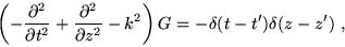
The solution to Eq.(34)
is the retarded Green's function, a unique scalar field, whose domain
extends over all four Rindler sectors. One accommodates the cylindrical
symmetry of the coordinate geometry by representing the scalar
field in terms of the appropriate eigenfunctions, the Bessel harmonics
 , for the Euclidean
  -plane:
 |
(36) |
where  satisfies
 |
(37) |
and
This Green's function is unique, and it is easy to show[#!HOW_TO_FIND_IT!#] that
 |
(38) |
This means that is non-zero only inside the future of the source
event  , and vanishes identically everywhere else. The
function
, and vanishes identically everywhere else. The
function  is defined on all four Rindler
sectors. However, our interest is only in those of its coordinate
representatives whose source events lie Rindler sectors
is defined on all four Rindler
sectors. However, our interest is only in those of its coordinate
representatives whose source events lie Rindler sectors  or
or  ,
,
and whose observation events lie in Rindler sector  ,
,
For these coordinate restrictions the two coordinate representatives
of , Eq.(38), are
and
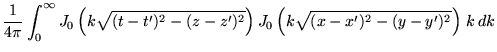
These two coordinate representatives give rise to the corresponding
two representatives of the unit impulse response, Eq.(36),
 |
(41) |
This integral expression is exactly what is needed to obtain the
radiation field from bodies accelerated in and/or . However,
in order to ascertain agreement with previously established knowledge,
we shall use the remainder of this subsection to evaluate the sum and
the integral in Eq.(41) explicitly.
It is a delightful property of Bessel harmonics that the sum over  can be evaluated in closed form[#!Sommerfeld!#]. This property is the Euclidean plane
analogue of what for spherical harmonics is the spherical addition
theorem. One has
can be evaluated in closed form[#!Sommerfeld!#]. This property is the Euclidean plane
analogue of what for spherical harmonics is the spherical addition
theorem. One has
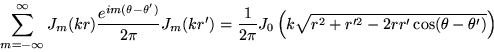 |
(42) |
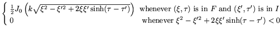
Inserting this result, as well as Eqs.(39) or (40)
into Eq.(41) yields the two unit impulse response functions with
sources in (upper sign) and (lower sign)
whenever
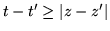 and zero otherwise.
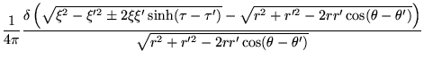
The spread-out amplitudes of this linear superposition interfere
constructively to form a Dirac delta function response. Indeed,
using the standard representation
and zero otherwise.
The spread-out amplitudes of this linear superposition interfere
constructively to form a Dirac delta function response. Indeed,
using the standard representation
for this function, one finds that
whenever  is in the future of
  .
This is the familiar causal response in due to a unit impulse event in
or in .
.
This is the familiar causal response in due to a unit impulse event in
or in .
Next: Full Scalar Radiation Field
Up: RADIATION: MATHEMATICAL RELATION TO
Previous: RADIATION: MATHEMATICAL RELATION TO
Ulrich Gerlach
2001-10-09