Geometrical Clocks

Time and space acquire their meaning from measurements, i.e. identifications of a relationship by means of a unit that serves as a standard of measurement. The measurement process we shall focus on is based on the emission, reflection, and reception of radar pulses generated by a standard geometrical clock.

Such a clock consists of a pair of Fourier compatible radar units, say, A and B. Their reflective surfaces form the two ends of a one-dimensional cavity with its evenly spaced spectrum of allowed standing wave modes in between. The operation of the geometrical clock hinges on having an electromagnetic pulse travel back and forth between the reflective ends of the cavity. The back and forth travel rate is determined by the separation between the cavity ends. This rate need not, of course, be constant in relation to the atomic clocks carried at either end. A geometrical clock with mutually receding ends would exemplify such a circumstance.

The definition of a geometrical clock is therefore this: it is a one-dimensional cavity

• whose bounding ends are Fourier compatible and
• which accommodates an electromagnetic pulse bouncing back and forth between the left and right end of the cavity.

This bouncing action forms the tick-tock events of the clock. If the cavity is expanding inertially, these events are located at

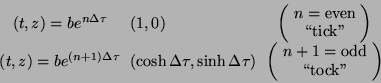$$\begin{array}{clc} (t,z)=be^{n\Delta\tau}&(1,0)& \left( \be... ...trm{odd}\\ \textrm{\lq\lq tock''} \end{array} \right) \end{array}$$ (2)

along the two straight world lines of radar units A and B in spacetime sector $F$. Here

$$e^{\Delta\tau}=k_{AB}$$

is the Doppler frequency shift factor and $\Delta\tau$ is the fixed comoving separation between A and B. The constant $b$ is the Minkowski time when the geometrical clock strikes zero.

For a clock with ends subjected to accelerations $1/b$ and $1/be^{\Delta\tau}$, the ticking events are located at

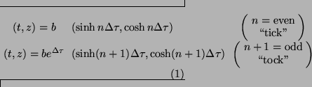
along the two hyperbolic world lines of A and B in boost-invariant sector $I$. Here

$$e^{\Delta\tau}=k_{AB}$$

is the pseudo-gravitational frequency shift factor between them, and $\Delta\tau$ is the boost time between a ``tick'' and a ``tock''.

The spacetime history of such clocks and their bouncing pulses are exhibited in Figures 2 and 3.

Figure 2: Spacetime history of an inertially expanding clock and the null trajectories of trains of emitted and received pulses (light lines) whose emission and reception is controlled by the internal pulse (heavy line) bouncing back and forth between A and B.

Figure 3: Spacetime history of an accelerated clock and the null trajectories of trains of emitted and received pulses (light lines) whose emission and reception is controlled by the internal pulse (heavy line) bouncing back and forth between A and B.

To serve its purpose, a geometrical clock AB emits and receives pulses of radiation. When the internal pulse strikes radar unit A its transmitter and its receiver are turned on only for the duration of the pulse. This causes A to emit a pulse and to register the reception of a pulse from the outside, if there is one coming. When the internal pulse has bounced back to B, an analogous emission and reception process takes place at radar unit B. It follows that that the tick-tock action of the internally bouncing clock pulse determines a set of external pulses moving to the right and to the left. The history of these pulses together with the clock that controls them is depicted by Figures 2 and 3 for an inertially expanding and accelerating clock respectively.