Anticanonical tropical del Pezzo cubic surfaces contain exactly 27 lines

Web page for the paper by María Angélica Cueto and Anand Deopurkar

The computational results in this web page were obtained using the software package SAGE 6.9 and special implementations done by the authors in Python. The sage outputs are stored as .sobj files and plain text files (whenever possible).

This material is based upon work supported by the National Science Foundation under Grant Number DMS 1700194. Any opinions, findings, and conclusions or recommendations expressed in this material are those of the author(s) and do not necessarily reflect the views of the National Science Foundation.

All scripts and outputs described in this page are available as a zip file here. CAVEAT: Some of the .sobj files may not load when working with earlier versions of SAGE. For this reason we also include plain text files of relevant outputs.

Jump to:

• Del Pezzo cubics and the root system E₆
• Equations for the anticanonical embedding X ⊂ P⁴⁴
• Computation of Yoshida and Cross functions
• The Bergman complex of the reflection arrangement of type E₆
• The Naruki fan
• Computation of tropical lines for non-apex cones in the Naruki fan
• Finding representatives of Cross functions for each Eckardt quintic
• Computation of tropical lines for the apex of the Naruki fan
• Boundary tree arrangements on anticanonical tropical cubic surfaces
• Computation of shifts and relevant Cross functions for each boundary tree.
• Boundary trees for the apex of the Naruki fan
• Boundary trees for the representatives of all non-apex cones of the Naruki fan
• Boundary tree arrangements from planar configurations
• The moduli space of stable tropical cubic surfaces.
• Combinatorics of anticanonically embedded tropical del Pezzo cubics
• References

§0. Del Pezzo cubics and the root system E₆

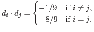
p ⟼ ([1: d₁(p): (d₁(p))³], …, [1: d₆(p): (d₆(p))³]).

The smooth del Pezzo surface X is obtained by blowing up six generic points in P². Via a Cremona transformation, we can assume these points lie in a cuspidal cubic, so their coordinates are determined by 6 generic points in the image of the map β. By abuse of notation, we write the ratio (x₁ / x₀) of coordinates for each of these 6 points as 6 parameters d₁,…, d₆. With this notation, the 6 generic points in the image of β become

P_i := (1: d_i: d_i³)     for i = 1,…,6.

The genericity of the points P₁, …, P₆ is determined by the following two conditions:

1. all points are distinct and no three points are colinear, which translates to non-vanishing of the following 20 expressions:

   (d_i - d_j) (d_i - d_k) (d_j - d_k) (d_i + d_j + d_k)       for 1 ≤ i < j < k ≤ 6 ;

2. the six points do not lie on a conic, which translates into the non-vanishing of the expression:

   (d₁ + d₂ + d₃ + d₄ + d₅ + d₆) Π_{1 ≤ i < j ≤ 6} (d_i - d_j).

In addition, we will assume that our del Pezzo surface X contains no Eckardt points. These points are defined by the condition of no three concurrent lines. These conditions are determined by 45 quintic equations which are conjugate to each other under the action of the Weyl group W(E₆). We call them Eckardt quintics. For example, the Eckardt quintic corresponding to the common intersection of the three lines associated to the tripartition {{1,2},{3,4},{5,6}} can be computed as the determinant of the following matrix:

• 6 Exceptional divisors E_i for i = 1,…,6;
• 15 Lines F_ij through 2 points P_i and P_j for 1 ≤ i < j ≤ 6;
• 6 Conics G_i passing through all 6 points but P_i for i = 1,…,6.

E_i = d_i - d₇   (1 ≤ i ≤ 6)  ,    F_ij = d_i + d_j+ d₇   (1 ≤ i < j ≤ 6) ,    G_i = (d₁ + … + d₇) - d_i   (1 ≤ i ≤ 6).

The following files encompass the information of the Root system E₆ and the action of the Weyl group on the parameters d₁,…, d₆ and hence on the anticanonical coordinates. They will be loaded loaded in most of the sage scripts given in sections below.

• Sage object containing the root lattice of the Root System E₆ encoded in sage: it is a saved version of the command RootSystem('E6').
• Sage object containing the ordered list of positive roots of E₆. The ordering of the positive roots varies among different versions of sage, and several of our scripts rely on a fixed choice of ordering. [Plain text version of the list containing one root per line]
• Plain text file containing the simple reflections of the Root System E₆ recorded above. It justifies the labelling in Figure 1. We view the root system E₆ inside E₇ by removing the node labeled as 7.



                     





• Sage script that transforms the positive roots of E₆ written as positive linear combinations of the simple roots α_i (i=1,…, 6) to linear expressions in the parameters d₁,…, d₆.
• Sage object: ordered list of positive roots of E₆ in terms of the parameters d₁,…, d₆. [Plain text version of the list containing one root per line] The simple roots α_i are expressed as follows:

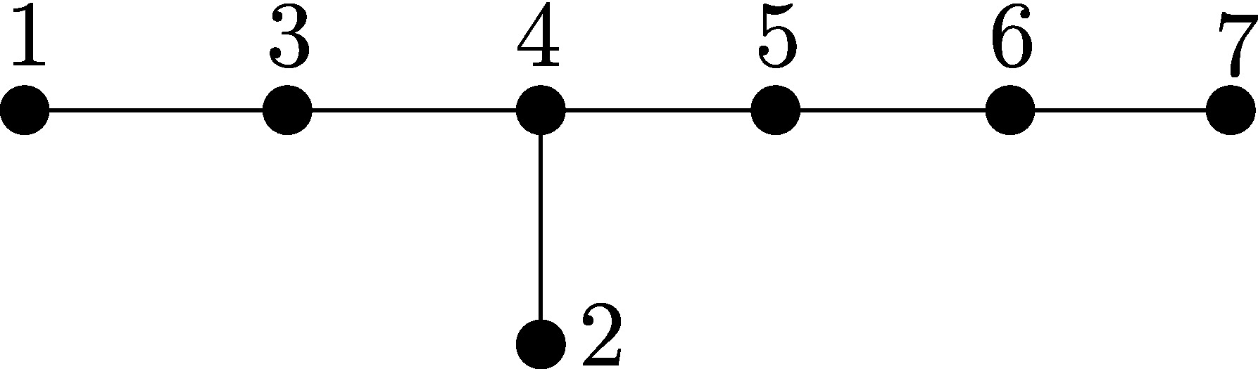
  α₁ = d₂ - d₁,     α₂ = d₁ + d₂ + d₃,       α₃ = d₃ - d₂,       α₄ = d₄ - d₃,       α₅ = d₅ - d₄,       α₆ = d₆ - d₅.

  The simple roots for E₇ are obtained by adding α₇ = d₇ - d₆.


• Sage script containing the data of the ambient ring of the 45 anticanonical coordinates together with the action of W(E₆) on the parameters d₁,…, d₆, as well as the 45 anticanonical coordinates X_ij (i,j=1,…,6), and Y_ijklmn (where {{i,j},{k,l},{m,n}} is a tripartition of [6]). In Section §2 we modify the action to multiples of the anticanonical coordinates adapted to the Yoshida function.

§1. Equations for the anticanonical embedding

The ideal defining the del Pezzo cubics via the anticanonical embedding is generated by 270 (trinomial) linear equations cutting the 41-dimensional space of linear elements of the ideal sheaf defining X ⊂ P⁴⁴ together with a single binomial cubic equation. The equations are expressed in terms of the 45 anticanonical coordinates (products of three (-1) curves each) and are computed with sage. The computations yield Theorem 3.5 in the paper.

The following files give a list of 270 linear equations that are stable under the action of the Weyl group W(E₆) and span a 41-dimensional linear space:

• Sage script: computes the orbit of an element under the action of a group. Here, it is mainly used to compute the W(E₆)-orbit of any polynomial in the anticanonical coordinates and the 6 parameters d₁,…, d₆.
• Sage script that picks one between a polynomial and its negative a given list of polynomials. Most of our ideals are obtained starting from a polynomial and a group action and we use this script to simplify the list of generators by removing negatives.


• Sage script for computing the 270 trinomial linear equations.
• Sage output: 270 linear equations in anticanonical coordinates. The entries are polinomials in 6 parameters d₁,…, d₆. It is obtained by acting on the single equation

  (d₃-d₄) (d₁+d₃+d₄) X₂₁ - (d₂-d₄) (d₁+d₂+d₄) X₃₁ + (d₂-d₃) (d₁+d₂+d₃) X₄₁

  by W(E₆). [Output in plain text]
• Sage script for computing the 4-dimensional space of solutions to the 270 linear equations.
• Sage output: 4x45 matrix whose rows span the solution space of the 270 linear equations. The entries are polinomials in 6 parameters d₁,…, d₆. [Output in plain text: the entries are rational functions in the d's]

The following files certify that the cubic equation Y₁₂₃₄₅₆ Y₁₄₂₅₃₆ Y₁₆₂₃₄₅ - Y₁₂₃₆₄₅ Y₁₄₂₃₅₆ Y₁₆₂₅₃₄ vanishes on the del Pezzo cubic but not on the ambient P³ defined by the previous 270 linear equations:

• Sage script: checks that the cubic equation vanishes on the del Pezzo cubic and does no lie in the ideal generated by the 270 linear trinomials by specializing the 6 parameters d₁,…, d₆ at random integers. It also checks that the W(E₆)-orbit of the give cubic lies in the ideal spanned by input cubic and the 270 linear equations. This script requires some of the scripts from Section §0.
• Sage output: computes the orbit of the binomial cubic and one between all elements and their negatives withing this orbit. The resulting set contains 121 cubic trinomials obtained by picking one between a polynomial and its negative a given list of polynomials. [Output in plain text]

Back to Top

§2. Computation of Yoshida and Cross functions

Each of the 40 Yoshida functions can be written as a degree 9 square-free monomial in the positive roots of E₆. We prescribe an ordering of the roots and record the exponent vectors for all Yoshida functions in the Yoshida matrix.

• Sage script to compute the 40 Yoshida functions as monomials in the positive roots of E₆ up to sign as well as their exponent vectors.
• Sage object: expression of the 40 Yoshida functions as monomials in the positive roots of E₆.
• Sage output: Yoshida integer matrix of size 40 x 36. Each row of the Yoshida matrix encodes the exponent vectors for each Yoshida function in terms of the ordered list of positive roots of E₆ given above. [Output in plain text]
• Sage object: ordered dictionary of 80 signed Yoshida functions as monomials in the positive roots of E₆, where the first 40 values correspond to the rows of the Yoshida matrix, and the next 40 to their negatives. In particular, the values of this dictionary are {Yoshida₀, …, Yoshida₄₀, - Yoshida₀, …, - Yoshida₄₀}.

The choice of basis for the anticanonical global sections done in Section §1 is not well-adapted to the Yoshida functions. Indeed, the solution to the 270 linear equations are not rational functions in the Yoshidas. However, there is another basis that satisfies this property: we obtain it by multiplying each of the 45 anticanonical coordinates by the inverse of a suitable quintic polynomial in the 6 parameters d₁,…, d₆. In the remainder, we refer to these 45 Yoshida-adapted anticanonical sections as the anticanonical coordinates.

The choice of a quintic for each anticanonical coordinate is compatible with the action of W(E₆) and it relates to the existence of Eckardt points, as described in Section §0.

The product of an Eckardt quintic with four suitable positive roots of E₆ can be rewritten as a linear binomial in the Yoshida functions of the form Yoshida_i - Yoshida_j. For example:

(d₅-d₆) (d₁+d₅+d₆) (d₃-d₄) (d₁+d₃+d₄) quintic[X₂₁] = - Yoshida₃ + Yoshida₃₇.

The Weyl group W(E₆) acts on these binomial Yoshida expressions, and the resulting orbit has 135 elements, up to sign. These expressions are known as Cross functions in the literature [Lemma 4.4, CGL].

The Yoshida functions are not algebraically independent. Furthermore, the binomial expression above is not unique. There are precisely 4 ways of writing each binomial. For example:

Cross₁₁₆ = Yoshida₃ - Yoshida₃₇ = Yoshida₁₇ - Yoshida₆ = - Yoshida₂₈ + Yoshida₃₃ = - Yoshida₂₁ + Yoshida₅.

We rewrite the 270 linear equations from Section §1 that are satisfied by these new coordinates and whose coefficients are rational functions in the Yoshidas: more precisely, they are associated to the 135 Cross functions.

• Sage object containing the list of Eckardt quintics, indexed by each one of the old 45 anticanonical coordinates X₁₂ through Y₁₆₂₅₃₄. These quintics cut out the parameters giving del Pezzo cubics with Eckardt points: points were 3 exceptional curves meet (and the corresponding anticanonical triangles degenerates.)


• Sage script for computing the triples of four factors (products of four roots of E₆) associated to each Eckardt quintic polynomial in the 6 parameters d₁,…, d₆ that produce the 135 Cross functions, as well as the dictionary identifying the 135 Cross functions (and their negatives) with the list of four linear binomials in Yoshidas giving each Cross functions.
• Sage object containing the correspondences between the 135 Cross functions (and their negatives) and the 4 tuples of linear binomials in the Yoshida functions as shown above. [Output in plain text]
• Sage object: dictionary writing each of the 135 Cross functions as polynomials in the parameters d₁,…, d₆
• Sage object: a dictionary (indexed by the 45 anticanonical coordinates X₁₂,…,Y₁₆₂₅₃₄) containing the triples of four positive roots that give a Cross function when multiplied by each Eckardt quintic. Each entry is a quartic polynomial in the ds. [Output in plain text: each entry is factorized for visual convenience]


• Sage script that computes the action of the 6 generators of W(E₆) on all variables (parameters d₁,…, d₆, Yoshida-adapted anticanonical coordinates, Yoshida functions and Cross functions). The result is a dictionary. Each variable is considered in the Symbolic Ring.
• Sage object: a dictionary containing the action of the 6 generators of W(E₆) on all variables (parameters d₁,…, d₆, Yoshida-adapted anticanonical coordinates, Yoshida functions and Cross functions). [Plain text version of the dictionary].
• Sage object: a dictionary describing the above action on the Symbolic ring. This speeds up the action computations dramatically.


• Sage script that contains several functions involving conversions between Cross functions, Yoshidas and products of roots and Eckardt quintics, in addition to functions used to compute pairwise intersections of the (-1)-curves in X, and to compose the actions of elements of W(E₆). These are used in Section §6 below.

• Sage script that computes the 270 linear equations that are satisfied by the Yoshida-adapted anticanonical coordinates as well as a basis of the space of solutions. These 270 equations are obtained from a single one using the action of W(E₆). The input linear equation

  (d₅-d₆) (d₁+d₅+d₆) {(d₃-d₄)(d₁+d₃+d₄) quintic[X₂₁] X₂₁ - (d₂-d₄)(d₁+d₂+d₄) quintic[X₃₁] X₃₁ + (d₂-d₃)(d₁+d₂+d₃) quintic[X₄₁] X₄₁}

  can be rewritten in terms of the Yoshida functions as follows:

  (Yoshida₃ - Yoshida₃₇) X₂₁ - (Yoshida₂₀ - Yoshida₈) X₃₁ + (Yoshida₃ - Yoshida₅) X₄₁.

  We rewrite the input linear equation using the 135 Cross functions:

  Cross₁₁₆ X₂₁ - Cross₂ X₃₁ + Cross₁₉ X₄₁.

  This expressions allows us to easily compute the W(E₆)-orbit of the new linear equation and then converts each coefficient to a binomial expression in the Yoshidas. Notice that all 135 Cross functions appear as coefficients. Our choice of Yoshida binomial expressions for the 270 linear equations will be consistent: we pick the first entry of each tuple.
• Sage output: set of 270 linear equations that vanish on the cubic del Pezzo X in the Yoshida-adapted anticanonical coordinates, where the coefficients are Cross variables. [Output in plain text]
• Sage output: set of 270 linear equations that vanish on the cubic del Pezzo X in the Yoshida-adapted anticanonical coordinates, where the coefficients are linear binomials in the Yoshida functions. [Output in plain text]


• Sage output: 4x45 matrix whose rows span the solution space of the above 270 linear equations with coefficients that are linear binomials in the Yoshida functions. The entries are rational functions in the 40 Yoshidas. The matrix is computed from the corresponding solution matrix given as rational functions in the parameters d₁,…, d₆ using this Sage script.
  [Output in plain text: the entries are rational functions in the Yoshidas] [Output in plain text (containing only the non-zero entries): the entries are rational functions in the ds, factored for visual convenience]


• Sage script giving the cubic equation in the Yoshida-adapted coordinates satisfied by the cubic del Pezzo X. The result is:

  (Yoshida₈ - Yoshida₁₁) (Yoshida₅ - Yoshida₁₇) (Yoshida₂₀ - Yoshida₈) X₁₂ X₂₃ X₃₁ - (Yoshida₈ - Yoshida₃) (Yoshida₃ - Yoshida₃₇) (Yoshida₁₉ - Yoshida₂₄) X₁₃ X₂₁ X₃₂.

  The binomial expressions for the coefficients are chosen in a canonical way, as we did with the linear equations. The same cubic equation can be written in terms of Cross functions:

  Cross₉ Cross₁₀₇ Cross₂ X₁₂ X₂₃ X₃₁ - Cross₈₀ Cross₁₁₆ Cross₈₆ X₁₃ X₂₁ X₃₂.

By construction, the ideal defining the anticanonical embedding of the universal cubic surface is valid for generic choices of Yoshida functions. In order to tropicalize all cubic surfaces, we must certify that the ideal is generated by the 270 linear trinomial and the 120 binomial cubics as long as the Yoshida and Cross functions do not vanish. This is done in the next script, which also rewrites the 4×45 matrix spanning the P³ space of solutions of the 270 linear equations. Since one of the maximal minors is a Laurent monomial in Yoshida and Cross functions, the chosen basis is valid for the del Pezzo surfaces we are interested in.

• Sage script that rewrite the matrix recording the solution space of the 270 linear functions in terms of Yoshida and Cross functions, and checks that the binomial cubic written earlier does not vanish along this P³. We also check that the cubic restricted to this space is irreducible whenever the Yoshida and Cross functions do not vanish.


• Sage output: 4x45 matrix whose rows span the solution space of the above 270 linear equations with coefficients that are Laurent monomials in the Yoshida and Cross functions. [Output in plain text]

Back to Top

§3. The Bergman complex of the reflection arrangement of type E₆

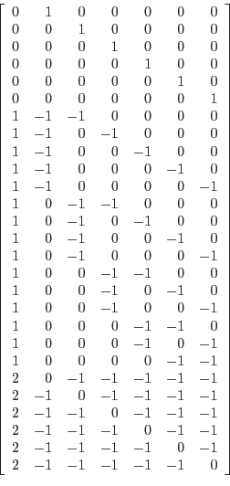
The reflection arrangement of type E₆ is the hyperplane arrangement defined by the 36 hyperplanes in R⁶ with defining equations given by all the 36 positive roots of the Root System E₆ written in terms of the basis {α_i}_{1 ≤ i ≤ 6} of simple roots. The ordered list "posRootsE6.sobj" of positive roots was mentioned already in Section §0. We are interested in the Bergman fan of the matroid associated to this arrangement.

The Bergman fan of a connected matroid M of rank k on the ground set [n] is the fan in Rⁿ over the geometric realization of the ordered complex of the proper part of the lattice of flats of the matroid. It has dimension k and all its cones contain the linear space spanned by the all-ones' vector. We consider the associated fan in R^n-1 ≅ Rⁿ / R 1. We can also realize this fan as the cone over the geometric realization of the nested set complex N(M, Irr) of the matroid associated to the minimal building set Irr consisting of all proper irreducible flats). Notice that the ground set is an irreducible flat since we assume the matroid is connected. However, the vector realizing the ground set will be the all-ones' vector which will be mapped to 0 in the quotient ambient space. We call this realization the Bergman complex.

As a combinatorial abstract object, the nested set complex N(M, Irr) consists of nested collections of flats in the geometric lattice of partially ordered flats of the matroid, ordered by inclusion. The vertices correspond to the irreducible flats, those which cannot be decomposed as a product. A collection F ⊂ Irr is nested if for every antichain {F₁,…, F_r} in F with r ≥ 2 the join flat F₁ ∨ F₂ ∨ … ∨ F_r does not belong to Irr ∪{ground set}, i.e. it is not a irreducible flat. Notice that the whole ground set is irreducible, since the matroid is connected. Notice that the join flat represents the subspace obtained by intersecting the given subspaces in the reflection arrangement of E₆. The vertices of the nested set complex are then realized in the Bergman complex as the 0-1 incidence vector of each irreducible flat, namely e_F := ∑ _{i ∈ F} e_i. We do not consider the maximal flat (the ground set of the matroid) since it will give rise to the all-ones vector 1 and it will become 0 in the quotient space Rⁿ / R 1. Higher dimensional cells in the Bergman complex are realized as convex combinations of vertices. We save the coordinates of all vertices and use this data to construct the Naruki fan in Section §4.

In what follows we focus our attention in the case of the reflection arrangement of E₆, although similar techniques apply to other connected matroids with group actions. By [BI, Theorem 3.1], there is a one-to-one correspondence between the lattice of flats of the reflection arrangement of E₆ (ordered by reverse inclusion) and the poset of parabolic subgroups of the Weyl group W(E₆). 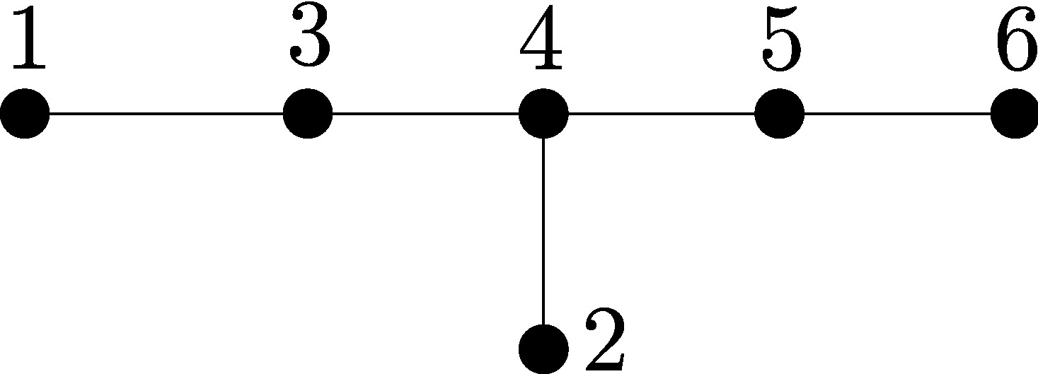Thus, we can characterize the flats by the root subsystems of E₆. There are exactly 15 types of such subsystems. An easy calculation confirms that, furthermore, each type is associated to exactly one W(E₆)-orbit of flats. Representatives for all possible subsystems are depicted in Figure 2. The codimension of each flat is the number of vertices of the associated root subsystem.

Our ordering of the 15 flat representatives is compatible with [RSS, Table 4]. The proper irreducible flats come from the 7 connected proper root subsystems of E₆, namely A₁, A₂, A₃, A₄, A₅, D₄ and D₅. Using this correspondence, we encode each flat as the set of all the positive roots of associated root subsystem as indicated in Figure 2. This description simplifies the distinction between different flats.

The Weyl group W(E₆) acts on the lattice of flats by permutation (it acts on the roots contained in each flat). We implement the action by means of the homomorphisms induced by simple reflections stored on the command RootLattice('E6') from Section §0. We are mainly interested in the action on the proper irreducible flats, since this determines the action on the vertices of the nested set complex, and hence on the Bergman complex.

To compute the action on the lattice of proper flats, we consider the action on the positive roots on a given flat F and take the linear span of the resulting set of roots. The comparison of a flat obtained by an action of an element of W(E₆) and the partial list of flats obtained by W(E₆)-actions is done on the linear span of the coordinate vectors of all the positive roots in the flat with respect to the basis of simple roots. This step is crucial since an element of the Weyl group might send a positive root to a negative one. If a new flat is encountered, it is encoded as usual, transforming all the coordinate vectors back to positive roots.

The construction of the nested set complex is done inductively, starting from all vertices and it makes heavy use of the group action as well as of its simplicial structure. Each vertex is associated to a proper irreducible flat. There are 750 of them and they are decomposed into 7 W(E₆)-orbits. Each cell in the complex is obtained by joining the flats associated to its vertices and checking if the join is irreducible or not. This step is performed by comparing the output flat to the stored list of all proper irreducible flats. We only consider the cell if the flat is not on this list. The join can be obtained by collecting all the positive roots contained in these flats and finding a minimal flat that contains them all. If there is more than one or if the flat is irreducible or not proper we discard the cell. This method allows us to find all higher dimensional cells containing a given one, by testing which vertices can be attached to it.

We use the action of W(E₆) on the lattice of proper flats (and hence on the collection of all proper irreducible flats) to construct a finite family (i.e. a dictionary with keys in [1,…, 6]) encoding the action of the 6 generators of W(E₆) on the set of vertices of the nested set complex. Each value of this family is a dictionary with keys and values in the interval [0,…,749]: the vertex indices obtained by acting with a give reflection on each vertex. This data is stored as a variable "dict" and then used to naturally extend the action to higher dimensional cells of the nested set complex. This information, together with the simplicial structure dramatically speeds up the construction of the nested set complex N(E₆, Irr) for three reasons:

1. Inductive step: We use the representatives of all cells of a fixed dimension l and the list of all vertices of the nested set complex to construct orbit-representative of all cells of dimension l+1. The new cells include representatives of all orbits but there could be more than one representative in the list. Our first input is the list of 7 representative vertices.
2. The action of W(E₆) on the cells of the nested set complex allows to build all the cells of fixed dimension l from a finite list containing representatives of all orbits of l-dimensional cells. The implementation does not requiere a single representative per orbit and in addition to computing all l-dimensional cells it outputs the orbit decomposition. This gives a list of representatives in dimension l+1 which we then feed back to the inductive step until l+1 reaches the dimension of the nested set complex (4 in our case).
3. We exploit the simplicial structure of the nested set complex and use information about the edge-vertex adjacency to reduct the candidate cells in each dimension. Rather than testing all vertices of the complex agains each low dimensional cone, we can restrict ourselves to vertices that form an edge with every since vertex in the cell. For this reason, we precompute the edges of the nested set complex and the adjacency conditions.

The following files contain the scripts, input and output files for the Bergman complex of the reflection arrangement of E₆ with respect to its collection Irr of proper irreducible flats. The output complex is simplicial. The calculation of both the Bergman complex and all the necessary inputs combined takes about 1 hour on a 2.4 GHz Intel(R) Core 2 Duo with 3MB cache and 2GB RAM. The time is split evenly between the calculation of adjacencies and the whole Bergman complex. The functions coded in the Sage scripts below can be used for other connected matroids with group actions on their lattice of flats if we choose a minimal building set (and remove the ground set) to construct the nested set complex.

• Sage script that computes the orbits of the flats of a matroid with ground set [n] under a group action given a suitable basis of the ambient space Rⁿ. The group action is encoded as a list of homomorphisms associated to its generators and the flat F is given as a set of all the elements of the ground set lying on the matroid. The action is performed on the coordinate vectors of the elements describing F with respect to the input basis. The file also contains a function that computes the list of coordinates of all elements on a set or a list with respect to an input basis.
  The computations return a list of all the flats in the orbit of F. The number of flats for E₆ on each orbit is encoded in the following vector:

  [36, 120, 270, 270, 720, 540, 45, 216, 540, 120, 1080, 27, 36, 216, 360]

  The orbits of proper irreducible flat correspond to the coordinates 1, 2, 4, 7, 8, 12, and 13 in the previous vector (the entries are labeled 1 through 15, in agreement with Figure 2.
• Sage script that provides a dictionary with the representatives of all the 15 W(E₆)-orbits of flats of the hyperplane arrangement associated to the root system E₆. In addition, this script generates and records the sorted lists of indices of all the positive roots contained in all the 750 proper irreductible flats, decomposed into 7 orbits. They are recorded as Sage objects and also in plain text form below.
• Compressed file of 15 sage objects corresponding to all the 15 orbits of proper flats. Each orbit is given as a list with two entries: first, the representative flat, and second, the list of all flats in the orbit. [Output in plain text (compressed file)]
• Compressed file of 7 sage objects containing to the sorted lists of indices of all positive roots contained in each W(E₆)-orbit of all proper irreducible flats. [Output in plain text (compressed file)]


• Sage script containing the necessary functions to compute the nested set complex N(M, Irr) of a matroid in terms of its building set Irr of (proper) irreducible flats. The resulting complex is simplicial. The bulk of the code takes advantage of the group action and builds the complex in an inductive fashion from a list of vertex representatives, certifying that at each step, each candidate new cell (obtained from a list of cell representatives and a list of potential vertices we could attach to each cell) does not correspond to a flat in Irr ∪{ground set}. It also allows to construct the list of edges and adjacencies among vertices of the complex. This information speed ups the calculation by dramatically reducing the number of candidate new cells in each step.


• Sage script that calculates input data required to compute the Bergman complex of E₆ as a complex in R³⁵ ≅ R³⁶ / R 1. More precisely, it provides:
  1. the list "rankE6" of flats of E₆: each entry of this list contains the indices of positive roots contained on each of the proper irreducible flats of that codimension. The first entry [] corresponds to the zero flat.
  2. the action of the simple reflections of W(E₆) on the vertices enconded as a list "dict" of 6 dictionaries (ordered in agreement with the ordering of the simple roots.)
• Sage script to compute the Bergman complex of the hyperplane arrangement associated to E₆. As intermediate steps, the script precomputes the 750 vertices and 17679 edges in the cell complex, and their orbit decomposition. In addition, it generates the 750 lists of all adjacent vertices to each vertex in the cell complex. This information is then saved as sage objects and plain text files.


• Sage object containing the list of all 7 W(E₆)-orbits of vertices in the Bergman complex of E₆. Each vertex is given as a list of one index in [0,749]. [Output in plain text]
• Sage object containing the list of all 24 W(E₆)-orbits of edges in the Bergman complex of E₆. Each edge is given as as ordered list of two indices in [0,749], corresponding to the vertices it connects. [Output in plain text]
• Sage object: a list of 750 entries containing information about the adjacencies among all vertices in the Bergman complex of E₆. The kth. entry is the ordered list of indices of all vertices adjacent to the kth. vertex. [Output in plain text (one list of adjacencies per line)]
• Sage script containing the list of six orbits of ray indices.


• Sage object: a list containing two entries. The first entry is the f-vector=[1, 750, 17679, 105930, 219240, 142560] of the Bergman complex of E₆ in TP³⁵, and the second is a list with 5 entries. The kth. entry contains the orbit decomposition of all cells in the Bergman complex of fixed dimension k. Each cell in the fan is given as an ordered list of the indices of all its vertices. The output required the precomputation of the vertices and their adjacencies. The number of orbits on each dimension equals [7, 24, 47, 49, 21]. We record the sizes of all orbits in each dimension:

      dim 0: [36, 120, 270, 45, 216, 27, 36],
      dim 1: [270, 360, 720, 1620, 540, 540, 2160, 216, 540, 540, 120, 1080, 720, 2160, 1080, 720, 540, 1080, 1080, 270, 540, 135, 432, 216],
      dim 2: [540, 2160, 1080, 810, 3240, 810, 3240, 2160, 1620, 270, 1620, 720, 3240, 2160, 6480, 3240, 2160, 360, 2160, 2160, 2160, 2160, 2160, 3240, 6480, 6480, 1620, 3240, 1080, 540, 540, 1620, 4320, 2160, 360, 2160, 4320, 4320, 1080, 2160, 2160, 4320, 2160, 1080, 540, 2160, 1080],
      dim 3: [3240, 1620, 540, 3240, 1620, 540, 1080, 2160, 6480, 6480, 6480, 6480, 6480, 2160, 1080, 1620, 3240, 3240, 810, 1620, 6480, 3240, 3240, 1620, 810, 6480, 3240, 2160, 6480, 12960, 12960, 3240, 6480, 6480, 12960, 6480, 4320, 2160, 2160, 4320, 2160, 6480, 3240, 12960, 6480, 4320, 2160, 8640, 4320],
      dim 4: [3240, 6480, 3240, 3240, 1620, 1620, 1620, 3240, 12960, 6480, 6480, 12960, 6480, 3240, 1620, 6480, 3240, 12960, 6480, 25920, 12960].



• Sage object: list of coordinates of all the 750 vertices viewed inside R³⁵ ≅ R³⁶ / R 1. We pick as representatives the vectors with last coordinate 0. The kth. entry gives the coordinates of the kth. vertex. [Output in plain text containing one vector per line]
• Compressed file of 5 plain text files: each file contains a variable (RepresentativesOrbitsAndCellsOfDimk) which is a list with two entries. The first one is the list of the orbit representatives of all cells of fixed dimension (k). The second entry is the orbit decomposition of all the cells of fixed dimension. The orbit representatives are the first entries on each orbit list. These files can also be loaded as sage files if needed, after changing their extension from '.txt' to '.sage'.

Back to Top

§4. The Naruki fan

As discussed in Section §2, the 40 Yoshida functions allow us to define a monomial map between two tori: (K^*)³⁶ and (K^*)⁴⁰. The coordinates on the domain are given by the 36 positive roots of E₆ and they map to the 40 degree 9 monomials in the positive roots. The map is compatible with the natural torus action on K^* on both sides as well as the action of the Weyl group W(E₆). We write

ϒ: (K^*)³⁶/K^* → (K^*)⁴⁰/K^*.

The image of this map is the (very affine) Yoshida variety Y ^o ⊂ (K^*)⁴⁰/K^*. It is the moduli space of marked cubic del Pezzo surfaces. Its tropicalization is the Naruki fan: a pure 4-dimensional fan in R³⁹ ≅ R⁴⁰ / R 1.
Tropicalizing the monomial map ϒ yields a linear surjective map trop(ϒ) between two fans: the Bergman fan Berg(E₆) of the reflection arrangement of E₆, constructed in Section §3, and the Naruki fan Trop(Y ^o). Both fans live in their respective tropical projective tori. The map is given by a 40×36 integer 0-1 matrix with nine ones per row and ten ones per column. We refer to it as the Yoshida matrix.

We use the linear map trop(ϒ), the simplicial structure of Berg(E₆) described in Section §3 and the action of the Weyl group W(E₆) to construct the Naruki fan and ensure that the linear map is a map of fans, i.e. it respects the polyhedral structure on both objects. For this, we start by mapping the rays of Berg(E₆) spanned by the 7 orbit-representatives of the vertices in the Bergman complex. Figure 2 describes these vertices and their images by colors. There are 4 types of images:

1. a ray associated to a vertex of type (a): it is the image of three orbits of vertices, labeled by the root subsystems A₁, A₄, and A₅. The action of W(E₆) gives a total of 36 vertices of type (a);
2. a ray associated to a vertex of type (b): it is the image of the single orbit of vertices labeled by the root subsystem A₂. The action of W(E₆) gives a total of 40 type (b) vertices;
3. a ray associated to a sum of two type (a) vertices, which we call type (a2) vertices: it is the image of the single orbit of vertices labeled by the root subsystem A₃. The action of W(E₆) gives a total of 270 vertices of type (a2);
4. all the vertices labeled by the root subsystems D₄ and D₅ map to multiples of the all-ones' vector, and hence to the origin in the tropical projective torus.

[[0, 1, 4, 36, 687], [0, 1, 4, 158, 691], [0, 1, 4, 158, 473], [0, 1, 4, 36, 473], [0, 1, 36, 165, 490], [0, 1, 36, 165, 687], [0, 1, 36, 471, 687], [0, 1, 156, 471, 687]  [0, 36, 159, 471, 687]]

The first two cells (in bold), have the additional properly that the orbits of the images of the remaining 7 representatives contain a cell whose image lies in the Naruki cone associated to one of these two cells. The union of the orbits of these two types of cones describes the support of the Naruki fan, but the collection does not determine a fan structure. Indeed, several of the intersections are full-dimensional. The union of suitable representatives of these cells form two tetrahedra, meeting along a commong face. Viewed in R³⁹, these are [0, 1, 4, 29] and [0, 1, 4, 36]. These are precisely the types (aaaa) and (aaab) from [RSS2]. We record the five vectors in the Bergman fan yielding the five generators of maximal cone representatives in the Naruki fan.

v₀   = [1, 0, 0, 0, 0, 0, 0, 0, 0, 0, 0, 0, 0, 0, 0, 0, 0, 0, 0, 0, 0, 0, 0, 0, 0, 0, 0, 0, 0, 0, 0, 0, 0, 0, 0, 0],
v₁  = [0, 1, 0, 0, 0, 0, 0, 0, 0, 0, 0, 0, 0, 0, 0, 0, 0, 0, 0, 0, 0, 0, 0, 0, 0, 0, 0, 0, 0, 0, 0, 0, 0, 0, 0, 0],
v₄  = [0, 0, 0, 0, 1, 0, 0, 0, 0, 0, 0, 0, 0, 0, 0, 0, 0, 0, 0, 0, 0, 0, 0, 0, 0, 0, 0, 0, 0, 0, 0, 0, 0, 0, 0, 0],
v₂₉ = [0, 0, 0, 0, 0, 0, 0, 0, 0, 0, 0, 0, 0, 0, 0, 0, 0, 0, 0, 0, 0, 0, 0, 0, 0, 0, 0, 0, 0, 1, 0, 0, 0, 0, 0, 0],
v₃₆ = [1, 0, 1, 0, 0, 0, 0, 0, 0, 1, 0, 0, 0, 0, 0, 0, 0, 0, 0, 0, 0, 0, 0, 0, 0, 0, 0, 0, 0, 0, 0, 0, 0, 0, 0, 0],
v₁₅₈= [1, 1, 0, 0, 0, 0, 0, 0, 0, 0, 0, 0, 0, 0, 0, 0, 0, 0, 1, 0, 0, 0, 0, 1, 1, 1, 0, 0, 0, 0, 0, 0, 0, 0, 0, 0].

n₀   = [0, 0, 0, 0, 0, 0, 1, 0, 0, 0, 0, 0, 0, 0, 0, 0, 0, 0, 0, 0, 1, 0, 1, 1, 0, 0, 1, 0, 0, 0, 1, 0, 0, 0, 0, 1, 1, 1, 1, 0],
n₁   = [0, 1, 0, 0, 1, 0, 0, 0, 0, 0, 0, 1, 0, 0, 0, 0, 0, 0, 1, 0, 0, 1, 1, 0, 0, 0, 1, 0, 0, 0, 0, 0, 0, 0, 0, 0, 0, 1, 1, 1],
n₄   = [0, 1, 1, 0, 0, 0, 0, 0, 0, 0, 0, 0, 0, 0, 0, 0, 1, 0, 1, 0, 0, 0, 1, 0, 0, 1, 0, 0, 0, 0, 1, 1, 0, 0, 0, 1, 0, 0, 1, 0],
n₂₉  = [0, 1, 0, 0, 0, 0, 0, 0, 0, 0, 0, 0, 0, 0, 0, 0, 0, 0, 1, 1, 0, 0, 0, 0, 0, 0, 1, 1, 1, 1, 1, 0, 0, 0, 0, 1, 0, 1, 0, 0],
n₃₆  = [1, 1, 1, 1, 1, 1, 1, 1, 1, 0, 1, 1, 1, 0, 0, 0, 1, 1, 1, 0, 1, 1, 3, 1, 0, 1, 1, 0, 0, 0, 1, 1, 0, 0, 0, 1, 1, 1, 1, 1],
n₁₅₈= [1, 3, 2, 1, 1, 1, 1, 1, 1, 1, 1, 1, 1, 1, 1, 1, 2, 1, 3, 2, 1, 1, 2, 1, 1, 2, 2, 2, 2, 2, 3, 2, 1, 1, 1, 3, 1, 2, 2, 1].

As shown in [RSS2], the overlaps mentioned earlier can be described as the maximal cells in the baricentric subdivision of the type (aaaa) cell and the induced subdivision on the second type of cell (aaab). Following [RSS2], we call them (aa₂a₃a₄) and (aa₂a₃b). We record the five spanning rays:

a   = [0, 0, 0, 0, 0, 0, 1, 0, 0, 0, 0, 0, 0, 0, 0, 0, 0, 0, 0, 0, 1, 0, 1, 1, 0, 0, 1, 0, 0, 0, 1, 0, 0, 0, 0, 1, 1, 1, 1, 0],
a₂ = [0, 1, 0, 0, 1, 0, 1, 0, 0, 0, 0, 1, 0, 0, 0, 0, 0, 0, 1, 0, 1, 1, 2, 1, 0, 0, 2, 0, 0, 0, 1, 0, 0, 0, 0, 1, 1, 2, 2, 1],
a₃ = [0, 2, 1, 0, 1, 0, 1, 0, 0, 0, 0, 1, 0, 0, 0, 0, 1, 0, 2, 0, 1, 1, 3, 1, 0, 1, 2, 0, 0, 0, 2, 1, 0, 0, 0, 2, 1, 2, 3, 1],
a₄ = [1, 4, 2, 1, 2, 1, 2, 1, 1, 1, 1, 2, 1, 1, 1, 1, 2, 1, 4, 2, 2, 2, 4, 2, 1, 2, 4, 2, 2, 2, 4, 2, 1, 1, 1, 4, 2, 4, 4, 2],
b  = [1, 1, 1, 1, 1, 1, 1, 1, 1, 0, 1, 1, 1, 0, 0, 0, 1, 1, 1, 0, 1, 1, 3, 1, 0, 1, 1, 0, 0, 0, 1, 1, 0, 0, 0, 1, 1, 1, 1, 1].

The following files compute the fan structure of the Naruki fan:

• Sage script that computes the Naruki fan from the Bergman fan E₆ and ensure that the 40×36 0-1 matrix mapping the Bergman fan to the Naruki fan is a map of fans. The algorithm starts from the Bergman fan and the matrix and constructs the Naruki fan as a set: it is the union of the images of the maximal cones C from Berg(E₆). We realize this image as the cone spanned by the images of the corresponding rays in C. We use the action of the Weyl group to reduce the computation to the image of the 21-orbit representatives of maximal cones in the Bergman fan. Our findings show that the Naruki fan is the union of the W(E₆)-orbits of Yoshida_map([0,1,4,36]) and Yoshida_map([0,1,4,29]). These cones are of type (aaaa) and (aaab).
  Once the above set description of the Naruki fan is given, it goes over the list of all the cones and refines the structure by checking overlaps between cones and adding the rays of the overlap (a polyhedron) to the list of rays in the Naruki fan. These rays are obtained from a baricentric subdivision of cone (aaaa) and the induced subdivision of (aaab). The rays added are (a₂), (a₃) and (a₄).
• Sage script that verifies that the tropicalization of the Cross functions do not produce any subdivision of the Naruki fan.
• Sage script that computes orbit representatives for cells in the Naruki fan, and their spanning rays.
• Sage object: the apex of R⁴⁴.
• Sage script containing the data and the functions to compute overlaps of cones.


• Sage object: Yoshida integer matrix of size 40 x 36 (from Section §2. Each row of the Yoshida matrix encodes the exponent vectors for each Yoshida function in terms of the ordered list of positive roots of E₆ given above. [Output in plain text]
• Sage object: a dictionary containing all 678 rays of the Naruki fan. They are obtained as the images of all 750 rays of the Bergman fan under the tropical Yoshida map trop(ϒ) and removing those for which this image is the zero-vector. The indices are compatible with the indices of the 750 vertices in Berg(E₆). [Output in plain text (one vector per line, including the corresponding index)]
• Sage object: list containing the maximal cone representatives [0,1,4,36,687] or [0,1,4,158,691] in the Naruki fan, the coordinates of each spanning ray in R₄₀ and the maximal cones in the Bergman fan whose image lies in these two cone representatives.
• Sage object: list 'max_orbit1' containing the list of ray indices of maximal cones in the Bergman fan that are in the orbit of [0,1,4,36,687].
• Sage object: list 'max_orbit2' containing the list of ray indices of maximal cones in the Bergman fan that are in the orbit of [0,1,4,158,691].
• Sage object: list 'max1_overlaps' containing cones in the Bergman fan that are in the orbit of [0,1,4,36,687] or [0,1,4,158,691] but whose image overlaps with the image of [0,1,4,36,687].
• Sage object: list 'max2_overlaps' contains cones in the Bergman fan that are in the orbit of [0,1,4,36,687] or [0,1,4,158,691] but whose image overlaps with the image of [0,1,4,158,691].
• Compressed file: each file is a Sage object describing the corresponding orbit-representative of cell in the Naruki fan, e.g. "aCell.sobj" contains an orbit representative of an (a)-type cell. Our choice of representatives is compatible with the inclusion of cells.
• Compressed file: each file is a Sage object describing the rays of the corresponding cell in the Naruki fan (see the previous item). [Output in plain text (compressed file)]

Back to Top

§5.Computation of tropical lines for non-apex cones in the Naruki fan

Several steps are required to show that there are no tropical lines in Trop(X) other than the 27 lines at infinity.

• The labels of each cell of the Naruki fan indicate how many rays of each type (a or b) are needed. For example, the top cell "aa2a3b" consists of a ray a, a sum of two type-a rays (a2), a sum of three type-a rays (a3) and a b ray. These cells comes from a baricentric subdivision of the top cells (aaaa) the induced subdivision of the cells (aaab) appearing in [RSS2]. There is one cell type on each W(E₆)-orbit.
• Each cell yields a polyhedral cone in R⁴⁵, recorded as a Sage object (column 3 of the table).

• Sage script that calculates a list of 27 quintuples of points in K⁴⁵ given by 45 rational functions in the Yoshidas. Each rational function factorizes as a product of Yoshidas and Cross functions, potentially with negative exponents. Each quintuple allows to compute the 5 boundary points of the potential non-boundary tropical lines associated to the corresponding extremal curve.


• Sage object: dictionary corresponding to the node E₁ ∩ F₁₂.
• Sage object: the 27 quintuples of points associated to the 27 extremal curves. The file contains a dictionary of 27 quintuples with keys E1,…,G6. Each value is a 5x45 (classical) matrix in terms of Yoshida functions representing the 5 points obtained as the vertices of the triangle with that particular exceptional curve. [Output in plain text (compressed file)]
• Sage script that computes both the expected and true coordinates of the 5 boundary points of the potential tropical lines on Trop(X) indexed by the 27 extremal curves. These points are defined as the expected and true valuations of 5 points at infinity described above, using the data of a relative interior point on each cell in the Naruki fan to input the valuation of the parameters d₁,…, d₆. Whenever a valuation cannot be determined, we write the corresponding entry as a "None." Each entry in columns 4 and 5 of Table 1 contains a Sage object file, with a list of 27 arrays of size 5 x 45 with values in {R}∪{"+Infinity"}∪{"None"}.
  
  Note: The columns of the matrices are ordered lexicographically, namely,

  [X₁₂, X₁₃, X₁₄, X₁₅, X₁₆, X₂₁, X₂₃, X₂₄, X₂₅, X₂₆, X₃₁, X₃₂, X₃₄, X₃₅, X₃₆, X₄₁, X₄₂, X₄₃, X₄₅, X₄₆, X₅₁, X₅₂, X₅₃, X₅₄, X₅₆, X₆₁, X₆₂, X₆₃, X₆₄, X₆₅, Y₁₂₃₄₅₆, Y₁₂₃₅₄₆, Y₁₂₃₆₄₅, Y₁₃₂₄₅₆, Y₁₃₂₅₄₆, Y₁₃₂₆₄₅, Y₁₄₂₃₅₆, Y₁₄₂₅₃₆, Y₁₄₂₆₃₅, Y₁₅₂₃₄₆, Y₁₅₂₄₃₆, Y₁₅₂₆₃₄, Y₁₆₂₃₄₅, Y₁₆₂₄₃₅, Y₁₆₂₅₃₄]

  In particular, column 0 of each matrix corresponds to the X₁₂ entry of the corresponding tropical node.
  
• Sage script containing all the functions necessary to compute the 5×45 matrices of the expected and true coordinates of the 5 boundary points of the potential tropical lines on Trop(X) indexed by the 27 extremal curves.
• Sage script: Script that computes a singular 3x3 tropical minors of a fixed triple of boundary points in a given potential tropical line indexed by an extremal curve. The coordinates involved have entries that lie in {R}∪{"+Infinity"}. These singular minors indicate that the 5 boundary points cannot lie in a tropical line in TP⁴⁴.
• Sage script that generates a singular 3x3 minors of each tropical matrix of boundary points in a potential tropical line labeled by each one of the 27 extremal curve. Using this we construct the sage objects appearing in the rightmost column of the table below.

Table 1 below contains all necessary files to rule out all 27 potential non-boundary tropical lines on the corresponding tropical del Pezzo cubics for every cell representative, with the exception of type a. For the latter, the method allows to reduce the labels of the potential tropical lines to 15 candidates, namely, the ones indexed by the extremal curves [E₅, F₅₆, F₃₆, E₆, F₄₅, G₃, F₃₄, E₄, F₁₂, G₅, F₃₅, E₃, F₄₆, G₄, G₆]. We treat these cases in Table 2.

The following table contains all files necessary to rule out from the cone of type a the 15 remaining non-boundary tropical lines, namely the ones indexed by the extremal curves [E₃, E₄, E₅, E₆, F₁₂, F₃₄, F₃₅, F₃₆, F₄₅, F₄₆, F₅₆, G₃, G₄, G₅, G₆]. The data was generated by this Sage script. We write the monomials (A/B)³ as a monomial in the 16 Yoshida functions Y₅ and Y₁₇ through Y₃₁ (encoded as as Sage object.)

Throughout the table, the cone is aCell.sobj. In all cases, the indicated tropical minor is singular assuming expected valuations of all its entries. However, the entries involved in each minor may have unexpected valuation, so we must study the entries in the 5x45-matrix of rational Yoshida functions. We indicate the vanishing, non-vanishing, and terms with possible unexpected valuation with a "-", a "*", and a "?", respectively. In all the cases, there are only two entries with "?" and they indicate the presence of non-monomial factors. We let A and B be the non-monomial part of each of these two entries. We verify that A/B is a product of positive roots in W(E₆) and its cube is a monomial in the Yoshida functions, hence their ratio has the expected valuation. Therefore, unexpected valuations will not change the number of terms realizing the minimum valuation and the tropical 3×3-minor will be non-singular.

The A and B can be read off from the family of matrices pds.sobj. The family of matrices pds is indexed by extremal curves. Each matrix in the family is indexed by rows (0 to 4) and columns by the 45 anticanonical triangles (labeled by X₁₂,…,Y₁₆₂₅₃₄, arranged lexicographically, and stored in anticanonical_keys.sobj).

For example, in the first row of the table, we have:

1. A = product of non-monomial factors in pds[E5][1][keys[14]]
2. B = product of non-monomial factors in pds[E5][2][keys[14]].

Once the data of the 27 tropical non-singular minors for the baricenter of each cone is provided, it remains to certify that the same minors are non-singular along the relative interior of each cone. The following script verifies this is the case. We use the matrices without Nones for all combinations (coneName, extremal), since even for the 15 problematic cases involving the cone (a), the difference between the expected and true valuations is the same for the relevant entries of these 15 matrices.

• Sage script that generates the data of minimizing terms, and non-Infinity terms of each 3×3 minor, and certifies the minimum is attained once for every point in the relative interior of the corresponding cone.
• Sage object: dictionary 'dataForMinors' containing the information of 3 rows, 3 columns, all non-'+Infinity' terms appearing the the tropicalization of the corresponding 3×3 minors, and the index corresponding to the minimum value once evaluated at the baricenter of the corresponding cone. For example, typing 'dataForMinors['b'][E1]' gives:

  ([0, 1, 2], [2, 8, 21], (1, [2, 4], {1: -3*Yoshida1 + 4*Yoshida10 + 2*Yoshida12 - Yoshida13 - 2*Yoshida14 + Yoshida15 + 2*Yoshida16 + 8*Yoshida17 + 2*Yoshida18 - Yoshida19 + 4*Yoshida21 - 6*Yoshida22 + 2*Yoshida23 + 2*Yoshida25 - Yoshida26 - Yoshida27 - 3*Yoshida28 - Yoshida29 + 2*Yoshida30 - 3*Yoshida31 - 2*Yoshida33 + 2*Yoshida34 + 2*Yoshida37 + 3*Yoshida38 - 2*Yoshida39 + Yoshida4 - 4*Yoshida5 - 3*Yoshida6 - 4*Yoshida9,
  2: Yoshida0 - 3*Yoshida1 + 2*Yoshida10 + 2*Yoshida12 - Yoshida13 - 3*Yoshida14 + 2*Yoshida15 + 2*Yoshida16 + 7*Yoshida17 + Yoshida18 + 3*Yoshida21 - 4*Yoshida22 + 2*Yoshida23 - Yoshida26 - Yoshida27 - 2*Yoshida28 - Yoshida29 + 2*Yoshida30 - 3*Yoshida31 - 2*Yoshida33 + 2*Yoshida34 + Yoshida37 + 4*Yoshida38 - 2*Yoshida39 + Yoshida4 - 3*Yoshida5 - 3*Yoshida6 - 3*Yoshida9,
  4: Yoshida0 - 4*Yoshida1 + 2*Yoshida10 + 2*Yoshida12 - Yoshida13 - 2*Yoshida14 + Yoshida15 + 4*Yoshida16 + 8*Yoshida17 + Yoshida18 + 3*Yoshida21 - 5*Yoshida22 + 2*Yoshida23 + Yoshida25 - Yoshida26 - Yoshida27 - 2*Yoshida28 - Yoshida29 + 2*Yoshida30 - 3*Yoshida31 - 3*Yoshida33 + 2*Yoshida34 + 2*Yoshida37 + 3*Yoshida38 - Yoshida39 + 2*Yoshida4 - 5*Yoshida5 - 3*Yoshida6 - 4*Yoshida9}))

  This indicates that the tropical minor with rows [0,1,2] and columns [2,8,21] has three non-'+Infinity' terms with indices 1, 2 and 4. The mininum is attained for the index 1.

Back to Top

§6. Finding representatives of Cross functions for each Eckardt quintic

The computation of the potential extra tropical lines in Trop(X_Yoshidas) where val(Yoshidas) is the apex in the Naruki fan requires prior knowledge of the expected valuation of all 135 Cross functions. This is done by picking generic examples of parameters d₁, …, d₆ yielding on the relative interior of each face of the two maximal cone representatives of the Naruki fan. We choose the baricenter as the random sample point for each cone (including the apex). For example, a sample representative for the cone (a₂a₄) and (aa₂a₃b) are given by the integer linear combinations a₂ + a₄, and a + a₂ + a₃ + a₄, respectively.
As representatives of vectors in the Bergman fan in the preimage of the five spanning rays of the two maximal cell representatives of the Naruki fan we choose

v_a   = [1, 0, 0, 0, 0, 0, 0, 0, 0, 0, 0, 0, 0, 0, 0, 0, 0, 0, 0, 0, 0, 0, 0, 0, 0, 0, 0, 0, 0, 0, 0, 0, 0, 0, 0, 0],
v_a2 = [1, 1, 0, 0, 0, 0, 0, 0, 0, 0, 0, 0, 0, 0, 0, 0, 0, 0, 0, 0, 0, 0, 0, 0, 0, 0, 0, 0, 0, 0, 0, 0, 0, 0, 0, 0],
v_a3 = [1, 1, 0, 0, 1, 0, 0, 0, 0, 0, 0, 0, 0, 0, 0, 0, 0, 0, 0, 0, 0, 0, 0, 0, 0, 0, 0, 0, 0, 0, 0, 0, 0, 0, 0, 0],
v_a4  = [2, 2, 0, 0, 0, 0, 0, 0, 0, 0, 0, 0, 0, 0, 0, 0, 0, 0, 1, 0, 0, 0, 0, 1, 1, 1, 0, 0, 0, 0, 0, 0, 0, 0, 0, 0],
v_b   = [1, 0, 1, 0, 0, 0, 0, 0, 0, 1, 0, 0, 0, 0, 0, 0, 0, 0, 0, 0, 0, 0, 0, 0, 0, 0, 0, 0, 0, 0, 0, 0, 0, 0, 0, 0].

• Sage script that computes dictionaries of valid parameters d₁, …, d₆ in the univariate polynomial ring Q[t] with least-order valuation for any point in the Bergman fan of E₆ (i.e. prescribed valuations for all 36 positive roots). All output examples are certified. The formula depends on the nature of the sample point (i.e in the fiber of which maximal cone representative of the Naruki fan it lies). The two formulas agree on the overlaps.
• Sage object: dictionary of parameters for positive dimensional faces of the (aa2a3a4) cone representative. [Output in plain text]
• Sage object: dictionary of parameters for positive dimensional faces of the (aa2a3b) cone representative. [Output in plain text]

Since ratios between Cross functions associated to a fixed Eckardt quintic have determined valuation (its cube is a monomial in Yoshida functions), we need only work with 45 of the 135 quintics (one for each triple associated to each quintic). The order of the Cross functions is such that these triples are labeled Cross_3k, Cross_3k+1, and Cross_3k+2 for k =0,…,44.
We use the parameters d₁, …, d₆ for each cone constructed earlier to search the 45 Cross functions where the expected valuation is attained generically. This strategy succeeds for all quintics except X₅₃ and its associated Cross functions Cross₁₅, Cross₁₆ and Cross₁₇. For these three Cross function, the expected valuation is not realized for the baricenter of four cones: (aa2a4), (aa4), (a2a4) and (a4). Throught our computations, we choose the following 45 Cross functions and write the remaining 90 as products of a reference Cross function and cube roots of Yoshidas:

[Cross₀, Cross₃, Cross₆, Cross₉, Cross₁₂, Cross₁₅, Cross₁₈, Cross₂₁, Cross₂₄, Cross₂₈, Cross₃₀, Cross₃₃, Cross₃₇, Cross₄₁, Cross₄₂, Cross₄₅,
Cross₄₈, Cross₅₁, Cross₅₄, Cross₅₇, Cross₆₀, Cross₆₃, Cross₆₆, Cross₆₉, Cross₇₃, Cross₇₆, Cross₇₈, Cross₈₁, Cross₈₄, Cross₈₇, Cross₉₀,
Cross₉₃, Cross₉₇, Cross₉₉, Cross₁₀₂, Cross₁₀₅, Cross₁₁₀, Cross₁₁₁, Cross₁₁₄, Cross₁₁₇, Cross₁₂₀, Cross₁₂₃, Cross₁₂₆, Cross₁₂₉, Cross₁₃₂]

• Sage script that computes the expected and true valuations for all 135 Cross functions per cone in the Naruki fan, picks a suitable Cross function from each triple associated to each Eckardt quintic and writes the remaining two Cross valuations as a linear combination of Yoshida functions (with scalars in 1/3 Z.) The method chooses expected valuations by exploiting the four ways of writing a Cross function as a difference of Yoshidas. Whenever these four values yield ties (so the true valuation becomes 'None'), we pick the largest one (from the values at the baricenter of the cone) as our expected valuation for the given Cross function. The valuations are recorded as the fourth column of Table 4. The ratios are recorded as a dictionary called 'dictionary_cross_ratios'.


• Sage object: dictionary 'tropical_dict_cross_ratios' of ratios of pairs of Cross functions associated to each Eckardt quintic as monomials in cube roots of Yoshida functions. The denominator is always a member of the list of Relevant Cross functions. For example, dictionary_cross_ratios[Cross16] has value:

  (Cross15, Yoshida20*Yoshida21*Yoshida22^2*Yoshida27*Yoshida29^3/(Yoshida17^3*Yoshida18*Yoshida26^2*Yoshida30*Yoshida5)

  where each Yoshida function should be interpreted as its cube root.
• Sage object: dictionary 'val_cross_to_yoshidas' of tuples of possible valuations for each Cross function on each cone representative in the Naruki fan arising from each expressions of this cross function as a difference of Yoshidas. Whenever there is a tie in their valuation, we record 'None'. Sample values:

  val_cross_to_yoshidas['aa2a3a4'][Cross30] = [Yoshida10, Yoshida3, Yoshida7, Yoshida0],
  val_cross_to_yoshidas['aa2a3a4'][Cross36] = [None, None, None, None].                          

• Sage object: dictionary 'dict_exp_cross_vals' of expected valuations of Cross functions for each cone in the Naruki fan. Each entry equals the valuation of suitable Yoshida function (since they do not vanish due to the lack of Eckardt points) [Output in plain text]
• Sage object: dictionary 'dict_true_cross_vals' of true valuations of Cross functions for each cone in the Naruki van. Each entry equals the valuation of suitable Yoshida function, or 'None' when the valuation cannot be determined [Output in plain text]
• Sage script that generates the dictionaries of all 135 tropical nodes for each extremal curve and each non-apex cone in the Naruki fan for both expected and true valuations of Cross functions. The script also computes the expected and true values at the baricenter of each cone. The later is obtained by a generic choice of parameters d₁, …, d₆. The outputs are seen in columns 6 through 9 of Table 4.
• Sage script that computes sample points for the baricenters (recorded) and 54 tropical matrices of size 10×45, four per extremal curve, and one family per cone representative in the Naruki fan specializing matrices in linear forms in Yoshida valuations to the sample points. The output files are presented in columns 8 and 9 on Table 4. The file also computes the differences between the true and specialized valuations.
  The first group encodes the specialization of the expected valuations to the point (the valuations of the 40 Yoshida functions) in each cone arising from the valuations on the Yoshidas corresponding to the baricenter of the cone (in column 5 of Table 4). The second group contains the true valuations arising from the sample parameters d₁, …, d₆ giving the baricenter of the cone. The entries on the last four groups are either integers or '+Infinity'. The coordinates of each node is given in lexicographically decreasing order Y₁₆₂₅₃₄, …, X₁₂.

Back to Top

§7. Computation of tropical lines for the apex of the Naruki fan

Tropical cubic surfaces associated to the apex (0-dimensional cell) of the Naruki fan include those obtained from assigning trivial valuation to the field K. We provide necessary and sufficient conditions on the valuations of the Cross functions that determine when each of the 27 five t-uples of boundary points are tropically collinear.

• Sage script that computes necessary and sufficient conditions on the valuations of the Cross functions that determine when each the 27 tuples of five boundary points is tropically collinear. Up to a shift, the resulting trees will have five rays and their unique vertex will be the origin in TP⁴⁴.
• Sage object: dictionary of 5 boundary points of a potential line after a global shift. Each column has either 0 or '+Infinity' entries or a collection of four distinct Cross valuations and one '+Infinity' entry. There are five Cross functions appearing overall on each dictionary.
• Sage object: dictionary encoding the global shift used in the previous item.
• Plain text file recording the shift point, the shifted tuple of five boundary points, the five Cross functions appearing. If the Cross functions have the same valuation, the five points are tropically collinear, and we record the 45 coordinates of the vertex of each extra tropical line.

• Sage script that shows that the 27 interior tropical lines in Trop(X) do not lift to algebraic curves in X in the trivially valued case.

A natural question that arises is the following: even though these 27 extra tropical lines do not lift to lines in the cubic surface, it might still be possible to lift them in pairs to a degree 2 curve in X. We show that this is not the case, since this curve will necessarilly contain the lifting of the 10 boundary points, and these points are not colinear: a numerical computation reveals that for generic choices of the 6 parameters d₁,…, d₆, the rank of the 10×45 matrix is 4. By Bézout's Theorem, such degree 2 curves are planar, so the 10 points cannot lie on a quadric curve in X.

• Sage script that takes the dictionary of quintuples of points in K⁴⁵ given by 45 rational functions in the Yoshidas computed with this Sage script, and verifies that their lifts give a 5⊗45 matrix of rank four. This verifies that no pair of distinct lines lifts to a plane residual conic. The script describes explicit conditions under which the 10⊗45 matrices obtained by joining boundery points of pairs as tropical rank 3.


• Sage object: dictionary 'dict_cross_ratiosInDs' of factorization of non-relevant Cross functions into relevant Cross functions and positive roots.
• Sage object: dictionary 'dictionary_cross_yoshidas_in_ds' of factorization of all Cross and Yoshida functions into relevant Cross functions and positive roots.
• Sage object: matrix 'matrixForE1InDsCross' of size 5×45 of boundary points for the extra tropical line indexed by E₁ in terms of relevant Cross functions, Yoshida functions and positive roots.
• Sage object: dictionary 'tenBoundaryPoints' of ten boundary points obtained by joining the 5 boundary points of pairs of extra tropical lines, where one of the indices is E₁
• Sage object: dictionary 'build10x45E1NonIntersectingPairs' that records the 10×45 matrix of boundary points for pairs of extra tropical lines, indexed by E₁ and an additional extremal curve not-intersecting E₁. We use it to show that the tropical matrix will have tropical rank 3 whenever the set of 10 relevant Cross functions arising from this pair all have valuation zero.
Sage object: dictionary 'build10x45E1IntersectingPairs' that records the 10×45 matrix of boundary points for pairs of extra tropical lines, indexed by E₁ and one of the 9 additional extremal curves intersecting E₁. We use it to show that the tropical matrix will have tropical rank 3 whenever the set of 9 relevant Cross functions arising from this pair have the same valuaion.

Back to Top

§9.Boundary tree arrangements on anticanonical tropical cubic surfaces

There are two types of trees for (aa2a3a4) cells, with 24 and 3 trees each. There are three types of trees for (aa2a3ab) cells, with 12, 12 and 3 trees. In what follows we describe how to compute the labelling for each cell by tropical convex hull computations. Section §10 discusses an alternative method, by considering planar configurations of six tropically generic points.

The computation of the 27 metric trees in Trop(X_Yoshidas) requires prior knowledge of the expected valuation of all 135 Cross functions and the choice of 45 relevant Cross functions, one for each Eckardt quintic. This was carried out in Section §6. Given the choice of 45 relevant Crosses, our next step is to determine the 10 nodes for each of the 27 lines, and their coordinatewise valuations in terms of the valuation of the 40 Yoshida functions and the 45 relevant Crosses. In turn, we must compute the valuations of the 135 nodes, as we move from cone to cone in the Naruki fan. Note that the valuations may be higher than the expected ones, so we must consider both the expected and true valuations.

The ordering of the rows corresponding to each matrix of leaves is given by the dictionary 'NodesOrdered'. We record its 27 values (one per exceptional curve):

The following scripts and files record this information:

• Sage script that computes the 135 classical nodes, the 10 relevant coordinates for the 10 nodes associated to a given extremal curve and the dictionaries of 10 tropical nodes per extremal curve. Each entry is either '+Infinity' or a linear function in the valuations of the 45 relevant Cross functions and the 40 Yoshida functions.
• Sage object: dictionary of correspondence between extremal curves and anticanonical triangles. For each extremal curve, we assign a dictionary of 0/1 values indexed by the 45 anticanonical triangles (we assign 1 if the indexing extremal curve lies in the triangle, and 0 otherwise.
• Sage object: dictionary 'infinityBlocks' of tuples of indices in [0,44] corresponding to the '+Infinity' valued anticanonical coordinates for all 10 nodes associated to each extremal curve (ordered lexicographically from X₁₂ to Y₁₆₂₅₃₄.) The first entry refers to the five common '+Infinity'-valued coordinates arising from the extremal curve itself. For example, infinityBlocks[E1] yields

  {F12: ([0, 1, 2, 3, 4], [5, 30, 31, 32]),      
  F16: ([0, 1, 2, 3, 4], [25, 42, 43, 44]),  
  F15: ([0, 1, 2, 3, 4], [20, 39, 40, 41]),  
  G4: ([0, 1, 2, 3, 4], [7, 12, 23, 28]),  
  G3: ([0, 1, 2, 3, 4], [6, 17, 22, 27]),  
  G2: ([0, 1, 2, 3, 4], [11, 16, 21, 26]),
  G6: ([0, 1, 2, 3, 4], [9, 14, 19, 24]),  
  G5: ([0, 1, 2, 3, 4], [8, 13, 18, 29]),  
  F14: ([0, 1, 2, 3, 4], [15, 36, 37, 38]), 
  F13: ([0, 1, 2, 3, 4], [10, 33, 34, 35])}
  

• Sage object: dictionary 'RelevantColumnsApex' of 10 anticanonical coordinates used to build the projection TP⁴⁴ → TP⁹ associated to each extremal curve. Each tuple is ordered according to the order of the 10 nodes from the dictionary 'NodesOrdered' computed with this Sage script and recorded at the beginning of this section. The choice is valid for all cones in the Naruki fan.

  {	E1:	[X23, X26, X61, X21, X31, X24, X51, X25, X32, X41],
  	E2:	[X15, X62, X52, X32, X16, X13, X42, X14, X12, X31],
  	E3:	[X53, X23, X16, X13, X63, X21, X43, X14, X12, X15],
  	E4:	[X13, X64, X12, X24, X54, X15, X16, X14, X21, X34],
  	E5:	[X12, X14, X16, X35, X45, X21, X13, X15, X65, X25],
  	E6:	[X13, X12, X21, X56, X14, X26, X16, X36, X15, X46],
  	F12:	[X13, X32, X36, X45, X31, X56, X46, X34, X23, X35],
  	F13:	[X21, X45, X32, X12, X24, X23, X56, X25, X46, X26],
  	F14:	[X36, X26, X23, X56, X35, X21, X42, X24, X25, X12],
  	F15:	[X25, X26, X24, X36, X46, X21, X23, X12, X34, X52],
  	F16:	[X25, X34, X26, X24, X12, X21, X35, X23, X62, X45],
  	F23:	[X31, X14, X21, X12, X15, X56, X16, X13, X46, X45],
  	F24:	[X16, X15, X56, X35, X41, X21, X14, X36, X13, X12],
  	F25:	[X16, X46, X36, X15, X34, X21, X12, X14, X13, X51],
  	F26:	[X15, X14, X21, X12, X35, X34, X16, X61, X45, X13],
  	F34:	[X16, X25, X26, X14, X13, X31, X12, X56, X15, X41],
  	F35:	[X31, X26, X24, X14, X13, X51, X16, X15, X46, X12],
  	F36:	[X14, X25, X15, X45, X12, X31, X13, X24, X61, X16],
  	F45:	[X13, X36, X12, X41, X14, X51, X26, X16, X15, X23],
  	F46:	[X25, X14, X41, X15, X12, X35, X16, X23, X13, X61],
  	F56:	[X14, X24, X16, X15, X23, X12, X61, X34, X13, X51],
  	G1:	[X13, X16, X14, X62, X15, X12, X32, X52, X23, X42],
  	G2:	[X61, X51, X26, X21, X23, X41, X25, X31, X13, X24],
  	G3:	[X12, X61, X41, X35, X21, X34, X36, X51, X32, X31],
  	G4:	[X51, X46, X43, X45, X12, X21, X61, X42, X31, X41],
  	G5:	[X21, X51, X52, X56, X41, X53, X12, X54, X31, X61],
  	G6:	[X61, X12, X31, X65, X51, X21, X62, X41, X64, X63]}

• Sage object: dictionary 'NodesFromPds' of ten classical nodes for each extremal curve written solely in terms of Yoshida functions. Each entry takes value in the function field of Yoshida functions. The same information but with values in the Symbolic Ring is recorded by the dictionary 'newNodesSR' available also as a Sage object file.
• Sage object: dictionary 'all135NodesInYC' of all 135 classical nodes with entries that are Laurent monomials in Yoshida and Cross functions. The same dictionary but with values in the function field of Yoshida functions is recorded as a Sage object file.
• Sage object: dictionary 'NodesYCPerExtremal' of ten classical nodes per extremal curve whith coordinates in the function field of Yoshida and Cross functions. [Output in plain text]
• Sage object: dictionary 'tropical_dict_cross_ratios' of tropicalizations of cross valuations in terms of the valuations of the 45 relevant Cross functions and the 40 Yoshida functions.
• Sage object dictionary 'TropYCNodesv2' recording the tropicalization of all 135 classical nodes. Each of the 45 coordinates of each node is either '+Infinity' or a linear functions in the valuations of the 45 relevant Cross functions and the 40 Yoshida functions.

To determine the labelling and metric structure on the 27 boundary trees we must compute the tropical convex hull for the tuple of ten tropical nodes associated each tree for each cone. The combinatorial type on each tree is recorded by the vertices of the trees and the direction of the inward vector for each such vertex. The types are constant on the relative interior of each cone, and the metric structure is linear in the scalars of the 5 types of spanning rays: (a), (a₂), (a₃), (a₄), and (b).

Since Cross functions appear in the coordinates of the tropical nodes, it is expected that not all entries will be determined. For the apex, we see that all non-diagonal entries of the 27 10×10 matrices are indetermined (i.e. their are 'None' types.) A careful analysis shows that all columns of the 27 symbolic matrices have a common Cross valuation summand. For example, the nodes associated to E₁ have the following Cross summands in the entries for the 10 relevant columns X₂₃, X₂₆, X₆₁, X₂₁, X₃₁, X₂₄, X₅₁, X₂₅, X₃₂, and X₄₁ corresponding to the rows associated to the nodes of E₁ and the curves G₃, G₆, F₁₆, F₁₂, F₁₃, G₄, F₁₅, G₅, G₂ and F₁₄, respectively:

	X23	X26	X61	X21	X31	X24	X51	X25	X32	X41
G3	+Infinity	-Cross63	-Cross45	-Cross114	Cross78-Cross0	-Cross21	-Cross24	-Cross93	-Cross84	-Cross18
G6	-Cross105	+Infinity	Cross33 -Cross45	-Cross114	-Cross0	-Cross21	-Cross24	-Cross93	-Cross84	-Cross18
F16	-Cross105	Cross33-Cross63	+Infinity	-Cross114	-Cross0	-Cross21	-Cross24	-Cross93	-Cross84	-Cross18
F12	-Cross105	-Cross63	-Cross45	+Infinity	-Cross0	-Cross21	-Cross24	-Cross93	Cross9-Cross84	-Cross18
F13	Cross78-Cross105	-Cross63	-Cross45	-Cross114	+Infinity	-Cross21	-Cross24	-Cross93	-Cross84	-Cross18
G4	-Cross105	-Cross63	-Cross45	-Cross114	-Cross0	+Infinity	-Cross24	-Cross93	-Cross84	Cross42-Cross18
F15	-Cross105	-Cross63	-Cross45	-Cross114	-Cross0	-Cross21	+Infinity	Cross111-Cross93	-Cross84	-Cross18
G5	-Cross105	-Cross63	-Cross45	-Cross114	-Cross0	-Cross21	Cross111-Cross24	+Infinity	-Cross84	-Cross18
G2	-Cross105	-Cross63	-Cross45	Cross9-Cross114	-Cross0	-Cross21	-Cross24	-Cross93	+Infinity	-Cross18
F14	-Cross105	-Cross63	-Cross45	-Cross114	-Cross0	Cross42-Cross21	-Cross24	-Cross93	-Cross84	+Infinity

By translating the corresponding ten tropical nodes by suitable linear combinations of canonical basis elements of TP⁹ where the scalar of e_i cancels the common Cross summand of the ith. column, we obtain 27 shifted matrices of size 10×10 with only 5 Cross functions appearing. Each of these functions appears in symmetric entries of each matrix. For example, for the 10×10 matrix associated to E₁ we translate all ten tropical nodes by the point

(Cross₁₀₅, Cross₆₃, Cross₄₅, Cross₁₁₄, Cross₀, Cross₂₁, Cross₂₄, Cross₉₃, Cross₈₄, Cross₁₈) in TP⁹.

Once the 27 matrices of shifted tropical nodes have been computed, we can determine the labelling and combinatorial type of all 27 boundary metric trees in terms of the valuations of the 45 relevant Cross functions. Assuming their values to be 0, we obtain 27 star trees. As the valuations become higher than expected, we obtain trees with five bounded edges.

The combinatorial information used to describe each metric tree consists of a dictionary encoding the labelling of each of its 10 leaves together with a list of of tuples recording the leaves, vertices and their coordinates in TP⁹. Each leaf and vertex comes with two pieces of data:

• 1) A list of the indices of the all the 10 leaves whose paths meet at the given vertex. For example, a single index corresponds to a leaf, and a list of two corresponds to the vertex of a cherry.
• 2) A list of the relevant coordinates (with entries in the Symbolic Ring) for the given vertex. These are unique modulo a scalar multiple of the all-ones vector.
• 3) 'True' or 'False' entry depending on the vertex being a non-leaf or not.

Back to Top

§9.1 Computation of shifts and relevant Cross functions for each boundary tree.

The following files are used to determine this data:

• Sage script that computes the 27 10×10 matrices of shifted tropical nodes associated to each extremal curve, parameters corresponding to the difference between the expected and true valuations of the five Cross functions appearing on each shifted matrix.


• Sage object: dictionary 'CrossInBlocksForNodes' recording the Cross factors for each block of infinity entries associated to each node on each extremal curve. For example, typing 'CrossInBlocksForNodes[E1][F12]' gives:

  {Y123456: [-Cross57, -Cross57, -Cross57, +Infinity, -Cross57, -Cross57, -Cross57, -Cross57, -Cross57 + Cross9, -Cross57], Y123546: [-Cross81, -Cross81, -Cross81, +Infinity, -Cross81, -Cross81, -Cross81, -Cross81, -Cross81 + Cross9, -Cross81], Y123645: [-Cross97, -Cross97, -Cross97, +Infinity, -Cross97, -Cross97, -Cross97, -Cross97, Cross9 - Cross97, -Cross97], X21: [-Cross114, -Cross114, -Cross114, +Infinity, -Cross114, -Cross114, -Cross114, -Cross114, -Cross114 + Cross9, -Cross114]}

• Sage object: dictionary 'allCrossesPerExtremalP44Apex' of all Cross summands appearing on each of the 10×45 matrices of tropical nodes associated to each extremal curve, together with the corresponding location (i,j) in the matrix, where i = row number (in agreement with the order given by the dictionary 'PairsForExtremals'), and j = anticanonical coordinate indexing the corresponding columns. For example, the row 0 of the matrix E1 (corresponding to the leaf labeled G3) has Cross factors on the following 36 non-Infinity entries:

  (-Cross0 + Cross78, 0, X31), (-Cross3, 0, X45), (-Cross63, 0, X26), (-Cross12, 0, Y142635), (-Cross90, 0, X35), (-Cross18, 0, X41),
  (-Cross21, 0, X24), (-Cross97, 0, Y123645), (-Cross24, 0, X51), (-Cross132 + Cross78, 0, Y132546), (-Cross41, 0, Y152436),
  (-Cross45, 0, X61), (-Cross48 + Cross78, 0, Y132456), (-Cross51, 0, X65), (-Cross54, 0, Y152634), (-Cross57, 0, Y123456),
  (-Cross6, 0, Y162345), (-Cross66, 0, X56), (-Cross69, 0, Y162534), (-Cross73, 0, X46), (-Cross76, 0, X54), (-Cross81, 0, Y123546),
  (-Cross84, 0, X32), (-Cross102, 0, X34), (-Cross93, 0, X25), (-Cross60, 0, Y162435), (-Cross99, 0, X36), (-Cross87, 0, X52),
  (-Cross110, 0, X62), (-Cross114, 0, X21), (-Cross117 + Cross78, 0, Y132645), (-Cross120, 0, Y142536), (-Cross123, 0, X64),
  (-Cross126, 0, X42), (-Cross129, 0, Y142356), (-Cross30, 0, Y152346).

  All 45 relevant cross functions appear on each matrix.


• Sage object: dictionary 'allShiftedTNodesApex' of all 27 10×10 matrices recording the 10 tropical nodes associated to each extremal curve shifted by a suitable point in TP⁹. For example, allShiftedTNodesApex[E1] gives
  
  

  [	[	+Infinity	0	0	0	Cross78	0	0	0	0	0	]	,
  	[	0	+Infinity	Cross33	0	0	0	0	0	0	0	]	,
  	[	0	Cross33	+Infinity	0	0	0	0	0	0	0	]	,
  	[	0	0	0	+Infinity	0	0	0	0	Cross9	0	]	,
  	[	Cross78	0	0	0	+Infinity	0	0	0	0	0	]	,
  	[	0	0	0	0	0	+Infinity	0	0	0	Cross42	]	,
  	[	0	0	0	0	0	0	+Infinity	Cross111	0	0	]	,
  	[	0	0	0	0	0	0	Cross111	+Infinity	0	0	]	,
  	[	0	0	0	Cross9	0	0	0	0	+Infinity	0	]	,
  	[	0	0	0	0	0	Cross42	0	0	0	+Infinity	]	].

• Sage object: dictionary 'newNoneEntriesCrossFactorsApex' of tuples of locations (row,col) of shifted matrices with Cross valuation summands. For each pair (row, col), we provide the scalar and the associated Cross function. For example, newNoneEntriesCrossFactorsApex[E1] gives

  {(1, 2): [(1, Cross33)],    
  (2, 1): [(1, Cross33)],  
  (3, 8): [(1, Cross9)],    
  (4, 0): [(1, Cross78)],  
  (5, 9): [(1, Cross42)],  
  (6, 7): [(1, Cross111)],
  (7, 6): [(1, Cross111)],
  (8, 3): [(1, Cross9)],    
  (9, 5): [(1, Cross42)]} 
  

• Sage object: dictionary 'allCrossesApexPerExtremal' of lists of five Crosses appearing on each of the 27 10×10 matrices of shifted tropical matrices. More precisely:

  {	E1:	[Cross9, Cross33, Cross42, Cross78, Cross111],
  	E2:	[Cross21, Cross63, Cross93, Cross105, Cross114],
  	E3:	[Cross0, Cross84, Cross90, Cross99, Cross102],
  	E4:	[Cross3, Cross18, Cross28, Cross73, Cross126],
  	E5:	[Cross15, Cross24, Cross66, Cross76, Cross87],
  	E6:	[Cross37, Cross45, Cross51, Cross110, Cross123],
  	F12:	[Cross9, Cross57, Cross81, Cross97, Cross114],
  	F13:	[Cross0, Cross48, Cross78, Cross117, Cross132],
  	F14:	[Cross12, Cross18, Cross42, Cross120, Cross129],
  	F15:	[Cross24, Cross30, Cross41, Cross54, Cross111],
  	F16:	[Cross6, Cross33, Cross45, Cross60, Cross69],
  	F23:	[Cross6, Cross30, Cross84, Cross105, Cross129],
  	F24:	[Cross21, Cross41, Cross48, Cross60, Cross126],
  	F25:	[Cross69, Cross87, Cross93, Cross120, Cross132],
  	F26:	[Cross12, Cross54, Cross63, Cross110, Cross117],
  	F34:	[Cross28, Cross54, Cross57, Cross69, Cross102],
  	F35:	[Cross12, Cross15, Cross60, Cross81, Cross90],
  	F36:	[Cross37, Cross41, Cross97, Cross99, Cross120],
  	F45:	[Cross3, Cross6, Cross76, Cross97, Cross117],
  	F46:	[Cross30, Cross73, Cross81, Cross123, Cross132],
  	F56:	[Cross48, Cross51, Cross57, Cross66, Cross129],
  	G1:	[Cross0, Cross18, Cross24, Cross45, Cross114],
  	G2:	[Cross9, Cross84, Cross87, Cross110, Cross126],
  	G3:	[Cross15, Cross28, Cross37, Cross78, Cross105],
  	G4:	[Cross21, Cross42, Cross76, Cross102, Cross123],
  	G5:	[Cross3, Cross51, Cross90, Cross93, Cross111],
  	G6:	[Cross33, Cross63, Cross66, Cross73, Cross99]}

  
  We assign parameters g₀, …, g₄ to record the valuation of the five Cross functions appearing on each of the 27 shifted matrices. The expected shifted tropical nodes are obtained by setting these five parameters to equal zero. We record this as the dictionary 'newExpectedVBShiftedSymbMatricesApex'. The true shifted tropical nodes are encoded as the dictionary 'newTrueVBShiftedSymbMatricesApex' of matrices with non-diagonal entries with values in {0, g₀, …, g₄}. Sample output:
  
  

  newExpectedVBShiftedSymbMatricesApex[E1]		newTrueVBShiftedSymbMatricesApex[E1]
  [[+Infinity, 0, 0, 0, 0, 0, 0, 0, 0, 0],		[[+Infinity, 0, 0, 0, g3, 0, 0, 0, 0, 0],
  [0, +Infinity, 0, 0, 0, 0, 0, 0, 0, 0],		[0, +Infinity, g1, 0, 0, 0, 0, 0, 0, 0],
  [0, 0, +Infinity, 0, 0, 0, 0, 0, 0, 0],		[0, g1, +Infinity, 0, 0, 0, 0, 0, 0, 0],
  [0, 0, 0, +Infinity, 0, 0, 0, 0, 0, 0],		[0, 0, 0, +Infinity, 0, 0, 0, 0, g0, 0],
  [0, 0, 0, 0, +Infinity, 0, 0, 0, 0, 0],		[g3, 0, 0, 0, +Infinity, 0, 0, 0, 0, 0],
  [0, 0, 0, 0, 0, +Infinity, 0, 0, 0, 0],		[0, 0, 0, 0, 0, +Infinity, 0, 0, 0, g2],
  [0, 0, 0, 0, 0, 0, +Infinity, 0, 0, 0],		[0, 0, 0, 0, 0, 0, +Infinity, g4, 0, 0],
  [0, 0, 0, 0, 0, 0, 0, +Infinity, 0, 0],		[0, 0, 0, 0, 0, 0, g4, +Infinity, 0, 0],
  [0, 0, 0, 0, 0, 0, 0, 0, +Infinity, 0],		[0, 0, 0, g0, 0, 0, 0, 0, +Infinity, 0],
  [0, 0, 0, 0, 0, 0, 0, 0, 0, +Infinity]]		[0, 0, 0, 0, 0, g2, 0, 0, 0, +Infinity]]

  
  
• Sage object: dictionary 'badKeys' that records the rows with a Cross function for each anticanonically indexed column of each 10×45 matrix of tropical nodes. All the non-empty lists of rows have size 9, so only one entry of each undetermined column is completely determined: the one with '+Infinity' value.

Back to Top

§9.1 Boundary Trees for the apex of the Naruki fan.

The following files are used to determine this data:

• Sage script that computes the 27 10×10 matrices of shifted tropical nodes associated to each extremal curve, parameters corresponding to the difference between the expected and true valuations of the five Cross functions appearing on each shifted matrix, the tropical convex hulls of each tuple of 10 shifted tropical nodes, the labelling and metric structure on each boundary tree for the apex.
• Sage object: dictionary 'TreesInRG_Apex' of all 27 metric trees for the tropical cubic surface associated to the apex of the Naruki fan. Each tree has five internal edges (possibly of length zero). As an example, the relevant columns for the line E1 are [6, 9, 25, 5, 10, 7, 20, 8, 11, 15], i.e. the anticanonical coordinates X23, X26, X61, X21, X31, X24, X51, X25, X32, and X41 (for the nodes with [G3, G6, F16, F12, F13, G4, F15, G5, G2 and F14]). Typing the command 'TreesInRG_Apex[E1]' yields:
  
  

  ({0: G3, 1: G6, 2: F16, 3: F12, 4: F13, 5: G4, 6: F15, 7: G5, 8: G2, 9: F14},

  [([0], [+Infinity, 0, 0, 0, g3, 0, 0, 0, 0, 0], False),

  ([1], [0, +Infinity, g1, 0, 0, 0, 0, 0, 0, 0], False),

  ([2], [0, g1, +Infinity, 0, 0, 0, 0, 0, 0, 0], False),

  ([3], [0, 0, 0, +Infinity, 0, 0, 0, 0, g0, 0], False),

  ([4], [g3, 0, 0, 0, +Infinity, 0, 0, 0, 0, 0], False),

  ([5], [0, 0, 0, 0, 0, +Infinity, 0, 0, 0, g2], False),

  ([6], [0, 0, 0, 0, 0, 0, +Infinity, g4, 0, 0], False),

  ([7], [0, 0, 0, 0, 0, 0, g4, +Infinity, 0, 0], False),

  ([8], [0, 0, 0, g0, 0, 0, 0, 0, +Infinity, 0], False),

  ([9], [0, 0, 0, 0, 0, g2, 0, 0, 0, +Infinity], False),

  ([0, 1, 2, 3, 4, 5, 6, 7, 8, 9], [0, 0, 0, 0, 0, 0, 0, 0, 0, 0], True),

  ([6, 7], [0, 0, 0, 0, 0, 0, g4, g4, 0, 0], True),

  ([5, 9], [0, 0, 0, 0, 0, g2, 0, 0, 0, g2], True),

  ([3, 8], [0, 0, 0, g0, 0, 0, 0, 0, g0, 0], True),

  ([1, 2], [0, g1, g1, 0, 0, 0, 0, 0, 0, 0], True),

  ([0, 4], [g3, 0, 0, 0, g3, 0, 0, 0, 0, 0], True)])



• Sage object: dictionary 'NonLeavesAndDistancesForExtremalInRG_Apex' of bounded edges and edge lengths for each boundary metric tree or the apex of the Naruki fan. Vertices are encoded by lists of elements in {0, …, 9} following our earlier convention. Edges are encoded by their adjacent vertices. The edge lengths are given as absolute values of the parameters g₀, …, g₄, which are non-negative by construction. [Output in plain text]
  
  For example, typing the command NonLeavesAndDistancesForExtremalInRG_Apex[E1] yields:
  
  

  [([0, 1, 2, 3, 4, 5, 6, 7, 8, 9], [6, 7], abs(g4)),

  ([0, 1, 2, 3, 4, 5, 6, 7, 8, 9], [5, 9], abs(g2)),

  ([0, 1, 2, 3, 4, 5, 6, 7, 8, 9], [3, 8], abs(g0)),

  ([0, 1, 2, 3, 4, 5, 6, 7, 8, 9], [1, 2], abs(g1)),

  ([0, 1, 2, 3, 4, 5, 6, 7, 8, 9], [0, 4], abs(g3))].

  
  
• Sage object: dictionary 'nonGenericTreesLeafLabelingAndDistancesInRG_PerExtremal_Apex' recording the combinatorial and metric structure for each of the 27 metric trees in terms of the four parameters g₀, …, g₄. It also includes the Cross function associated to each parameter. [Output in plain text (compressed file)]

Back to Top

§9.2 Boundary Trees for the representatives of all non-apex cones of the Naruki fan.

We employ the 27 10×10 matrices of shifted tropical nodes associated to each extremal curve to compute the tropical convex hulls of each tuple of nodes. The expected valuation of all 45 relevant Cross functions in all 23 non-apex cone representatives are realized by sample generic choices of parameters d₁, …, d₆, with the exception of Cross₁₅ and the four cones (aa₂a₄), (aa₄), (a₂a₄) and (a₄). Suitable 3×3-minors on the matrices for the extremal curves E₅, F₃₅, G₃ confirm that the expected valuations are never realized. Furthermore, this computation determines a formula for the new expected valuation of this Cross function on these four cones, that agrees with that obtained from sample parameters. For each cone and each extremal curve, we determine the combinatorial and metric structures on the associated trees in terms of non-negative parameters g₀, …, g₄ accounting for the difference between the true and expected valuations of the five Cross functions appearing on each 10×10 matrix. Only 222 out of the 621 trees potentially arise from non-generic situations. The following files are used to determine all trees:

• Sage script that computes the 10×10 matrices of shifted tropical nodes associated to each extremal curve and each cone representative of the Naruki fan, the parameters corresponding to the difference between the expected and true valuations of the (up to) five Cross functions appearing on each shifted matrix, the tropical convex hulls of each tuple of 10 shifted tropical nodes, the labelling and metric structure on each boundary tree. We include both the outputs for the expected and true valuations of the Cross functions where a discrepancy can occur.


• Sage object: dictionary 'allShiftedTNodes' of all 27 10×10 matrices recording the 10 tropical nodes associated to each extremal curve, shifted by a suitable point in TP⁹. Each entry is a linear function in Yoshida and Cross valuations, or '+Infinity.' For example, allShiftedTNodes[E1][0] corresponding to the shift of the node (E1,G4) gives
  
  

  [	+Infinity,
  	Yoshida0 + Yoshida10 - 2*Yoshida12 + Yoshida17 - 2/3*Yoshida18 + Yoshida2 - 4/3*Yoshida20 + 5/3*Yoshida21 - 2/3*Yoshida22 - Yoshida24 + Yoshida25 + 2/3*Yoshida26 + 2/3*Yoshida27 - 2*Yoshida28 + Yoshida29 - Yoshida3 + 4/3*Yoshida30 + Yoshida31 - 2*Yoshida34 - Yoshida39 + Yoshida4 - 2/3*Yoshida5 + Yoshida6,
  	2*Yoshida0 + Yoshida10 - 2*Yoshida12 + 1/3*Yoshida18 - Yoshida19 + 2*Yoshida2 - 1/3*Yoshida20 + 8/3*Yoshida21 + 1/3*Yoshida22 + Yoshida25 - 1/3*Yoshida26 + 2/3*Yoshida27 - Yoshida28 + 2*Yoshida29 - Yoshida3 + 1/3*Yoshida30 - Yoshida31 - 2*Yoshida34 - Yoshida39 - 5/3*Yoshida5,
  	4*Yoshida0 + 2*Yoshida10 - Yoshida11 - 4*Yoshida12 + Yoshida17 + 1/3*Yoshida18 - 2*Yoshida19 + 2*Yoshida2 - 1/3*Yoshida20 + 11/3*Yoshida21 - 2/3*Yoshida22 + Yoshida25 - 1/3*Yoshida26 + 2/3*Yoshida27 - Yoshida28 + 2*Yoshida29 - 3*Yoshida3 + 4/3*Yoshida30 - Yoshida31 - 3*Yoshida34 - 2*Yoshida39 + Yoshida4 - 8/3*Yoshida5 + Yoshida6 + 2*Yoshida8,
  	Cross78 + 2*Yoshida0 + Yoshida10 - 2*Yoshida12 - 1/3*Yoshida18 - Yoshida19 + Yoshida2 - 2/3*Yoshida20 + 4/3*Yoshida21 - 1/3*Yoshida22 + 4/3*Yoshida26 - 2/3*Yoshida27 + Yoshida29 - Yoshida3 - 1/3*Yoshida30 + Yoshida31 - 2*Yoshida34 - Yoshida39 - 1/3*Yoshida5 + Yoshida8,
  	Yoshida0 + Yoshida10 - 2*Yoshida12 + Yoshida17 + 1/3*Yoshida18 + Yoshida2 - 1/3*Yoshida20 + 2/3*Yoshida21 - 2/3*Yoshida22 - Yoshida24 + 2/3*Yoshida26 + 2/3*Yoshida27 - Yoshida28 + Yoshida29 - Yoshida3 + 1/3*Yoshida30 + Yoshida31 - 2*Yoshida34 - Yoshida39 + Yoshida4 - 2/3*Yoshida5 + Yoshida6,
  	3*Yoshida0 + 2*Yoshida10 - 3*Yoshida12 - 1/3*Yoshida18 - Yoshida19 + 2*Yoshida2 + 1/3*Yoshida20 + 10/3*Yoshida21 - 1/3*Yoshida22 - 2/3*Yoshida26 + 1/3*Yoshida27 + 2*Yoshida29 - 2*Yoshida3 + 2/3*Yoshida30 - 3*Yoshida34 - 2*Yoshida39 + Yoshida4 - 7/3*Yoshida5 + Yoshida8,
  	4*Yoshida0 + 2*Yoshida10 - Yoshida11 - 4*Yoshida12 + Yoshida17 + 4/3*Yoshida18 - 2*Yoshida19 + 2*Yoshida2 + 2/3*Yoshida20 + 8/3*Yoshida21 - 2/3*Yoshida22 - 1/3*Yoshida26 + 2/3*Yoshida27 + 2*Yoshida29 - 3*Yoshida3 + 1/3*Yoshida30 - Yoshida31 - 3*Yoshida34 - 2*Yoshida39 + Yoshida4 - 8/3*Yoshida5 + Yoshida6 + 2*Yoshida8,
  	3*Yoshida0 + 2*Yoshida10 - 3*Yoshida12 + 2*Yoshida17 + 4/3*Yoshida18 - 2*Yoshida19 + 2*Yoshida2 - 1/3*Yoshida20 + 11/3*Yoshida21 - 5/3*Yoshida22 + Yoshida23 - Yoshida24 + Yoshida25 - 1/3*Yoshida26 + 2/3*Yoshida27 - 2*Yoshida28 + 2*Yoshida29 - 2*Yoshida3 + 4/3*Yoshida30 - Yoshida31 - 3*Yoshida34 - 2*Yoshida39 + Yoshida4 - 8/3*Yoshida5 + Yoshida8,
  	Yoshida0 + Yoshida10 + Yoshida11 - Yoshida12 + Yoshida2 + Yoshida21 + Yoshida29 - Yoshida3 + Yoshida31 - 2*Yoshida34 - Yoshida39 - Yoshida5	]



• Sage object (compressed files): dictionaries of all shifted Tropical Nodes where all cross variables with known valuations are replaced by the corresponding Yoshida. To reduce the size of the output, each dictionary is saved in a separate file.
• Sage object: dictionary 'newNoneEntriesCrossFactorsPerExtremalPerCone'of tuples of locations (row,col) of shifted matrices with Cross valuation summands with unknown valuations for each extremal curve and each cone of the Naruki fan. For each pair (row, col), we provide the scalar and the associated Cross function. For example, 'newNoneEntriesCrossFactorsPerExtremalPerCone[E6]['aa2a3a4']' gives

  {(0, 7): [(1, Cross37)], (7, 0): [(1, Cross37)]}.

  As with the apex, there is at most one Cross function per entry and all scalars equal 1. Furthermore, symmetric entries must have the same Cross function. There are 223 combinations of extremal curves and cones where the dictionary 'newNoneEntriesCrossFactorsPerExtremalPerCone[extremal][coneName]' is non-empty. The number of combinations with a given fixed number of Cross functions with unknown valuations is determined by the following data:

  {0: 398, 1: 146, 2: 42, 3: 30, 5: 5}.

• Sage object: dictionary 'dict_exp_PerExtremalPerCone' of true valuations of the five Cross functions appearing in the shifted matrix of tropical nodes associated to each extremal. These values depend on the choice of cone in the Naruki fan. When the valuation cannot be determined, we incorporate a parameter g_i to account for the potential difference between the expected and true valuations. For example, typing 'dict_exp_PerExtremalPerCone[E6]['aa2a3a4']' yields

  {Cross51: Yoshida2, Cross110: Yoshida29, Cross123: Yoshida31, Cross45: Yoshida1, Cross37: Yoshida34 + g0}

• Sage object (compressed files): dictionaries of all shifted Tropical Nodes where all appearances of cross variables are replaced by the corresponding values given by 'dict_exp_PerExtremalPerCone'. To reduce the size of the output, each dictionary is saved in a separate file.
• Sage object: dictionary 'dict_true_matrices_l0CoM' of shifted matrices of tropical nodes for each extremal curve at the baricenter of each cone in the Naruki fan for all 223 combinations where at least some Cross function has undetermined valuation. The keys of the dictionary are in triples 'tce' with values (number of parameters, cone Name, extremal curve). [Output in plain text]
  By construction, at least two (symmetric) entries of each matrix include some parameter g_i. The dictionary 'dict_expected_matrices_l0CoM' of matrices arising from expected valuations is obtained by specializing all parameters g_i appearing in each entry of 'dict_true_matrices_l0CoM' to be zero . For example, the key tce=(1,'a2a3a4',E1) yields:

  dict_expected_matrices_l0CoM[tce]		dict_true_matrices_l0CoM[tce]
  [[+Infinity, 10, 10, 10, 8, 9, 5, 9, 10, 5],		[[+Infinity, 10, 10, 10, g3 + 8, 9, 5, 9, 10, 5],
  [7, +Infinity, 3, 7, 1, 5, -2, 5, 3, -2],		[7, +Infinity, 3, 7, 1, 5, -2, 5, 3, -2],
  [10, 6, +Infinity, 6, 4, 5, 4, 5, 10, 4],		[10, 6, +Infinity, 6, 4, 5, 4, 5, 10, 4],
  [10, 10, 6, +Infinity, 4, 8, 1, 8, 6, 1],		[10, 10, 6, +Infinity, 4, 8, 1, 8, 6, 1],
  [14, 10, 10, 10, +Infinity, 9, 5, 9, 10, 5],		[g3 + 14, 10, 10, 10, +Infinity, 9, 5, 9, 10, 5],
  [-1, -2, -5, -2, -7, +Infinity, -10, -1, -5, -10],		[-1, -2, -5, -2, -7, +Infinity, -10, -1, -5, -10],
  [3, -1, 2, -1, -3, -2, +Infinity, -2, 2, -1],		[3, -1, 2, -1, -3, -2, +Infinity, -2, 2, -1],
  [7, 6, 3, 6, 1, 7, -2, +Infinity, 3, -2],		[7, 6, 3, 6, 1, 7, -2, +Infinity, 3, -2],
  [13, 9, 13, 9, 7, 8, 7, 8, +Infinity, 7],		[13, 9, 13, 9, 7, 8, 7, 8, +Infinity, 7],
  [2, -2, 1, -2, -4, -3, -2, -3, 1, +Infinity]]		[2, -2, 1, -2, -4, -3, -2, -3, 1, +Infinity]]

• Sage object: list 'badMinors' of all 3×3 non-singular tropical minors for each 10×10 matrix of true shifted tropical nodes with values in R[g₀, …, g₄] ∪ {'+Infinity'} associated to each extremal curve specialized at the baricenter of each Naruki cone. We only compute the minors for all combinations of extremal curves and cones whose matrix features at least one indeterminate g_i in it. There are 0, 34 or 40 bad minors for each such matrices.
  Whenever len(badMinors[tce])=0 for some valid key 'tce', we conclude that the parameters g_i can be 0, i.e. the corresponding Cross functions can have the expected valuations while preserving the tropical collinearity of the ten tropical nodes. Furthermore, we confirm that in all these cases, the Crosss functions involved generically achieve their expected valuation.
  All twelve remaining cases involve a parameter associated to Cross₁₅. The minor computation confirms that its expected valuation on the cones (aa₂a₄), (aa₄), (a₂a₄) and (a₄) is never achieved and we must therefore alter the original formula for its expected valuation. Table 4 records the minor on each combination (curve, cone) used to determine the new formula both at the corresponding baricenters and along all cones. All 12 cases yield the same value. [Output in plain text: all 12 relevant matrices with one bad minor per matrix to adjust the parameter associated to Cross₁₅]
  
  

  Table 4: Computing new expected valuations for Cross₁₅ on the cones (aa₂a₄), (aa₄), (a₂a₄) and (a₄) via tropical minors.

  Extr. Curve	Cone	Number param.	Number of bad minors	Rows	Cols	Minor at baricenter	Updated min. value for parameter
  E5	(aa2a4)	1	40	[1, 3, 6]	[0, 1, 3]	[ -2, +Infinity, -1 ] [ -9, -9, +Infinity ] [ -4, -4, g0 - 4 ]	g0 ↦ g0+1
  E5	(aa4)	1	40	[1, 3, 6]	[0, 1, 3]	[ -1, +Infinity, 0 ] [ -6, -6, +Infinity ] [ -2, -2, g0 - 2 ]	g0 ↦ g0+1
  E5	(a2a4)	1	40	[1, 3, 6]	[0, 1, 3]	[ -2, +Infinity, -1 ] [ -8, -8, +Infinity ] [ -4, -4, g0 - 4 ]	g0 ↦ g0+1
  E5	(a4)	1	40	[1, 3, 6]	[0, 1, 3]	[ -1, +Infinity, 0 ] [ -5, -5, +Infinity ] [ -2, -2, g0 - 2 ]	g0 ↦ g0+1
  F35	(aa2a4)	1	40	[2, 4, 5]	[0, 2, 4]	[ -2, +Infinity, 0 ] [ 2, 3, +Infinity ] [ -9, -8, g1 - 8 ]	g1 ↦ g1+1
  F35	(aa4)	1	40	[2, 4, 5]	[0, 2, 4]	[ -1, +Infinity, 1 ] [ 1, 2, +Infinity ] [ -6, -5, g1 - 5 ]	g1 ↦ g1+1
  F35	(a2a4)	1	40	[2, 4, 5]	[0, 2, 4]	[ -2, +Infinity, 0 ] [ 1, 2, +Infinity ] [ -8, -7, g1 - 7 ]	g1 ↦ g1+1
  F35	(a4)	1	40	[2, 4, 5]	[0, 2, 4]	[ -1, +Infinity, 1 ] [ 0, 1, +Infinity ] [ -5, -4, g1 - 4 ]	g1 ↦ g1+1
  G3	(aa2a4)	3	34	[2, 3, 7]	[0, 2, 3]	[ -6, +Infinity, -5 ] [ 2, 3, +Infinity ] [ -4, -3, g0 - 4 ]	g0 ↦ g0+1
  G3	(aa4)	3	34	[2, 3, 7]	[0, 2, 3]	[ -4, +Infinity, -3 ] [ 1, 2, +Infinity ] [ -2, -1, g0 - 2 ]	g0 ↦ g0+1
  G3	(a2a4)	5	34	[2, 3, 7]	[0, 2, 3]	[ -5, +Infinity, -4 ] [ 1, 2, +Infinity ] [ -4, -3, g0 - 4 ]	g0 ↦ g0+1
  G3	(a4)	5	34	[2, 3, 7]	[0, 2, 3]	[ -3, +Infinity, -2 ] [ 0, 1, +Infinity ] [ -2, -1, g0 - 2 ]	g0 ↦ g0+1



• Sage object: dictionary 'altered_dict_true_matrices' of matrices for the baricenter of each extremal curve and cone in the Naruki fan with updated values of parameters as given by column 8 of Table 4.
• Sage object: dictionary 'minorsToCheckVB0' of the triples (3 rows, 3 columns, minor) associated to the 12 bad minors on columns 5, 6 and 7 of Table 4. This information is used to update the expected valuation of Cross₁₅.
• Sage object: dictionary 'LinearIneqToCheck' of linear inequalities that the parameters corresponding to Cross₁₅ must satisfy arising from the 12 bad minors given by the rows and colums listed on Table 4. Here:
  

  minor0 =	submatrix[0][0]*submatrix[1][1]*submatrix[2][2],
  minor1 =	submatrix[1][0]*submatrix[2][1]*submatrix[0][2],
  minor2 =	submatrix[2][0]*submatrix[1][1]*submatrix[0][2],

  where submatrix corresponds to the 3×3 submatrix of shifted tropical nodes (with entries that are linear functions in Cross and Yoshida valuations). The shape of each minor is such that the there are only three values to compare: minor0, minor1 and minor 2. In agreement with the findings for the baricenter of the four relevant cones described in Table 4, a direct computation reveals that minor1=minor2 on the whole cone. Therefore, the linear inequality we must impose to guarantee the tropical minor is singular is minor0 ≥ minor1. Each value is a triple (0, minor1, minor0). The first entry of the triple is a placeholder confirming that all minors have the expected shape. A simple comparison, yields the following three inequalities (one per extremal curve) that are valid on the cones (aa₂a₄), (aa₄), (a₂a₄), (a₄) and its facets:
  
  

  E5:	2*Yoshida1 - Yoshida10 + Yoshida14 + Yoshida15 + Yoshida16 - 4*Yoshida17 + 2/3*Yoshida18 + 2*Yoshida2 + 7/3*Yoshida20 - 5/3*Yoshida21 + 2/3*Yoshida22 + Yoshida24 - Yoshida25 + 1/3*Yoshida26 + 1/3*Yoshida27 + Yoshida28 - Yoshida29 + Yoshida3 - 13/3*Yoshida30 - 2*Yoshida34 + Yoshida36 - Yoshida38 + Yoshida39 - 2*Yoshida4 + 2/3*Yoshida5 + Yoshida6 + z,
  F35:	-Yoshida0 + Yoshida1 + Yoshida10 + Yoshida14 - Yoshida15 - Yoshida17 - 1/3*Yoshida18 - Yoshida19 + 7/3*Yoshida20 - 5/3*Yoshida21 + 8/3*Yoshida22 + 2*Yoshida24 - Yoshida25 - 2/3*Yoshida26 + 1/3*Yoshida27 + 3*Yoshida28 - Yoshida3 - 7/3*Yoshida30 + 2*Yoshida34 - Yoshida36 - Yoshida38 - Yoshida39 + Yoshida4 - 4/3*Yoshida5 - Yoshida7 + z,
  G3:	-Yoshida11 + Yoshida12 - Yoshida15 - 2*Yoshida16 - 3*Yoshida17 + Yoshida20 + Yoshida21 + 3*Yoshida22 + Yoshida24 - Yoshida25 - Yoshida27 + Yoshida28 + 2*Yoshida29 + 2*Yoshida3 - Yoshida30 + 4*Yoshida32 - Yoshida33 + Yoshida36 - Yoshida37 - Yoshida39 - Yoshida4 - 3*Yoshida6 - 3*Yoshida7 + Yoshida8 + 2*Yoshida9 + z,

  
  where the variable z represents g0 for E5 and G3, and g1 for F35. [Output file in plain text]
  A direct computation reveals that these three inequalities agree. This is done by checking the baricenter of each cone and all its faces. We conclude that the difference between the true and the expected valuation is bounded below by the following expression:
  
  

  Cross15 - Yoshida32	≥		-2*Yoshida1 - 2*Yoshida2 - Yoshida3 + 2*Yoshida4 - 2/3*Yoshida5 - Yoshida6 + Yoshida10 - Yoshida14 - Yoshida15 - Yoshida16
  			+ 4*Yoshida17 - 2/3*Yoshida18 - 7/3*Yoshida20 + 5/3*Yoshida21 - 2/3*Yoshida22 - Yoshida24 + Yoshida25 - 1/3*Yoshida26
  			- 1/3*Yoshida27 - Yoshida28 + Yoshida29 + 13/3*Yoshida30 + 2*Yoshida34 - Yoshida36 + Yoshida38 - Yoshida39.



• Sage object: dictionary 'reldictCrossParamPerExtremalPerCone' of expressions for all parameters g_i for all 223 combinations of extremal curve and Naruki cones as linear expressions of valuations of all 45 relevant Cross and 40 Yoshida functions. For example, typing 'reldictCrossParamPerExtremalPerCone[E6]' yields:
  

  {'aa2a3a4': {g0: Cross37 - Yoshida34},
  'aa2a3': {g0: Cross37 - Yoshida34},
  'aa2a4': {g0: Cross37 - Yoshida34},
  'aa3a4': {g4: Cross123 - Yoshida39, g2: Cross51 - Yoshida39, g0: Cross37 - Yoshida34},
  'a2a3a4': {g0: Cross37 - Yoshida34},
  'aa3b': {g4: Cross123 - Yoshida39, g2: Cross51 - Yoshida39},
  'aa2': {g0: Cross37 - Yoshida34},
  'aa3': {g4: Cross123 - Yoshida39, g2: Cross51 - Yoshida39, g0: Cross37 - Yoshida34},
  'aa4': {g4: Cross123 - Yoshida39, g2: Cross51 - Yoshida39, g0: Cross37 - Yoshida34},
  'a2a3': {g0: Cross37 - Yoshida34},
  'a2a4': {g0: Cross37 - Yoshida34},
  'a3a4': {g4: Cross123 - Yoshida39, g2: Cross51 - Yoshida39, g0: Cross37 - Yoshida34},
  'ab': {g4: Cross123 - Yoshida39, g2: Cross51 - Yoshida39},
  'a3b': {g4: Cross123 - Yoshida39, g2: Cross51 - Yoshida39},
  'a': {g4: Cross123 - Yoshida39, g2: Cross51 - Yoshida39, g0: Cross37 - Yoshida34},
  'a2': {g0: Cross37 - Yoshida34},
  'a3': {g4: Cross123 - Yoshida39, g2: Cross51 - Yoshida39, g0: Cross37 - Yoshida34},
  'a4': {g4: Cross123 - Yoshida39, g3: Cross110 - Yoshida36, g2: Cross51 - Yoshida39, g1: Cross45 - Yoshida38, g0: Cross37 - Yoshida34},
  'b': {g4: Cross123 - Yoshida39, g2: Cross51 - Yoshida39}}
  

• Sage object: dictionary 'newdict_exp_PerExtremalPerCone' of true valuations for all five Cross functions appearing on the ten shifted tropical nodes of each extremal curve for all Naruki cones. For example, typing 'newdict_exp_PerExtremalPerCone[E5]['aa2a4']' yields:

   {Cross15: -2*Yoshida1 + Yoshida10 - Yoshida14 - Yoshida15 - Yoshida16 + 4*Yoshida17 - 2/3*Yoshida18 - 2*Yoshida2 - 7/3*Yoshida20 + 5/3*Yoshida21 - 2/3*Yoshida22 - Yoshida24 + Yoshida25 - 1/3*Yoshida26 - 1/3*Yoshida27 - Yoshida28 + Yoshida29 - Yoshida3 + 13/3*Yoshida30 + Yoshida32 + 2*Yoshida34 - Yoshida36 + Yoshida38 - Yoshida39 + 2*Yoshida4 - 2/3*Yoshida5 - Yoshida6 + g0,
    Cross24: Yoshida24,
    Cross66: Yoshida23,
    Cross76: Yoshida23,
    Cross87: Yoshida13}.

  This information is used to build 27 dictionaries 'allTrueShiftedTNodesPerCone' of all shifted Tropical Nodes where all appearances of cross variables are replaced by the adjusted values given by 'newdict_exp_PerExtremalPerCone'. We place this data as the third column of Table 5.

• Sage object: dictionary 'nonGenTrees' of the combinatorial types, vertex and leaf coordinates of all 223 metric trees where a discrepancy between expected and true valuations of relevant Cross functions may occur. Each vertex and leaf coordinate is written in terms of the scalars r₁, …, r₄ and (up to five) parameters g_i.


• Sage object: dictionary 'genNonLeavesAndDistancesInRG_PerExtremalPerCone' encoding the metric of all metric trees in the generic case (i.e. where the valuations of all Cross functions are the expected ones). Each edge lenght is a linear function of the non-negative scalars r₁, …, r₄. For example, the metric for the extremal curve E₁ on the two maximal cone representatives is:
  
  

  genNonLeavesAndDistancesInRG_PerExtremalPerCone[E1]['aa2a3a4']		genNonLeavesAndDistancesInRG_PerExtremalPerCone[E1]['aa2a3b']
  [([2, 6, 8, 9], [6, 9], abs(-r3 - r4)),		[([2, 6, 8, 9], [2, 4, 6, 8, 9], abs(-r2 - r3)),
  ([2, 6, 8, 9], [2, 4, 6, 8, 9], abs(-r2 - r3 - r4)),		([2, 6, 8, 9], [2, 6, 9], abs(-r4)),
  ([2, 6, 8, 9], [2, 8], abs(-r4)),		([6, 9], [2, 6, 9], abs(-r3)),
  ([1, 3, 5, 7], [5, 7], abs(-r3 - r4)),		([5, 7], [1, 5, 7], abs(-r3)),
  ([1, 3, 5, 7], [1, 3], abs(-r4)),		([2, 4, 6, 8, 9], [0, 1, 3, 5, 7], abs(-r1)),
  ([1, 3, 5, 7], [0, 1, 3, 5, 7], abs(-r2 - r3 - r4)),		([1, 3, 5, 7], [1, 5, 7], abs(-r4)),
  ([2, 4, 6, 8, 9], [0, 1, 3, 5, 7], abs(-r1))]		([1, 3, 5, 7], [0, 1, 3, 5, 7], abs(-r2 - r3))]



• Sage object: dictionary 'nonGenNonLeavesAndDistancesInRG_PerExtremalPerCone' encoding the metric of all 223 potentially non-generic metric trees (i.e. where the valuations of all Cross functions can be strictly the expected ones). [Output in plain text]
  Each value is a list of tuples with three entries. The first two are the end points of the edge (encoded as list of indices, following our earlier conventions). The last entry is the lattice distance between these two vertices (primitive vectors have length one). It is a linear function of the non-negative scalars r₁, …, r₄ and the parameters g₀, …, g₄. The combinatorial types for non-generic cases can be different than for the generic ones. For example, in the case of the extremal curve E₅ and the cone 'aa3a4' we have:
  
  

  genNonLeavesAndDistancesInRG_PerExtremalPerCone[E5]['aa3a4']		nonGenNonLeavesAndDistancesInRG_PerExtremalPerCone[E5]['aa3a4']
  [([1, 2, 4, 5], [4, 5], abs(-r4)),		[([0, 1, 2, 3, 4, 5, 6, 7, 8, 9], [1, 2, 4, 5], abs(r3 + r4)),
  ([1, 2, 4, 5], [0, 1, 2, 3, 4, 5, 6, 7, 8, 9], abs(-r3 - r4)),		([0, 1, 2, 3, 4, 5, 6, 7, 8, 9], [0, 6, 7, 8], abs(r3 + r4)),
  ([1, 2, 4, 5], [1, 2], abs(-r1 - r3 - r4)),		([0, 1, 2, 3, 4, 5, 6, 7, 8, 9], [3, 9], abs(g1)),
  ([0, 6, 7, 8], [7, 8], abs(-r4)),		([1, 2, 4, 5], [4, 5], abs(-r4)),
  ([0, 6, 7, 8], [0, 1, 2, 3, 4, 5, 6, 7, 8, 9], abs(-r3 - r4)),		([1, 2, 4, 5], [1, 2], abs(-r1 - r3 - r4)),
  ([0, 6, 7, 8], [0, 6], abs(-r1 - r3 - r4))]		([0, 6, 7, 8], [7, 8], abs(-r4)),
  		([0, 6, 7, 8], [0, 6], abs(-r1 - r3 - r4))]



• Sage object: dictionary 'nonGenericvsGenTreesLeafLabelingAndDistancesInRG_PerExtremalPerCone' of all combinatorial and metric data for each of the 621 extremal trees, for both generic and non-generic combinations (extremal curves, non-apex cone representative).

• Drawing of all 27 generic trees corresponding to the two maximal cone representatives


• Drawing of non-generic trees corresponding to the maximal cones among all 223 pairs (extremal, cone) with potential gaps between the true and expected valuations on some relevant Cross functions. The generic trees are recovered by setting parameters g_i.

Back to Top

§11. Boundary tree arrangements from planar configurations

Each line L on the cubic surface X comes with a natural 2-to-1 cover of P¹ with five marked points. The fiber over each such point consists of pairs of lines forming a tritangent plane with L. This map induces an involution on each line. The same is true after tropicalization. The following scripts checks that these involutions do not come from elements of the Weyl group W(E₆):

• Sage script to certify that the involution on each of the 27 trees do not come from an element of the Weyl group W(E₆). It also computes the action of each element of this group on the tuples of 27 lines, the parameters d₁,…, d₆, Yoshida functions, Cross functions and Yoshida-adapted anticanonical coordinates.
• Compressed file: Sage objects describing the action of all 51840 elements of the Weyl group W(E₆) on tuples of 27 lines, the parameters d₁,…, d₆, Yoshida functions, Cross functions and Yoshida-adapted anticanonical coordinates. The tuples are encoded as numbers corresponding to the lexicographic order of the 27 lines E₁,…, E₆, F₁₂,…, F₅₆, G₁,…, G₆.

By [RSS2, Theorem 4.4], each of the 27 metric trees and the labeling of its 10 leaves can be computed from a configuration of 6 generic points in TP². We set three of the points as the tropicalization of the three torus fixed points, namely P₁=(0:∞:∞), P₂=(∞:0:∞), P₃=(∞:∞:0). We choose the other three points in two ways, each one determining a configuration yielding one of the two maximal cells in the Naruki fan:

(aa2a3a4) Cell: p₄ = (-12:6:0), p₅ = (-17:4:0), p₆ = (0:0:0),    and    (aa2a3b) Cell: p₄ = (-10:10:0), p₅ = (2:5:0), p₆ = (0:0:0).

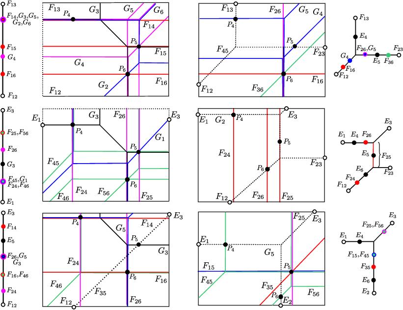
Nonetheless, we can use the action of the Weyl group W(E₆) and the information obtained from tropical convex hulls computations to determine the labellings on the missing three exceptional lines. The following scripts perform this task:

• Sage script that computes the Weyl group elements that send the labelling of each of the 27 trees on each maximal cone of the Naruki fan to those of the trees computed from the planar configurations in TP².
• Sage object: tuple of 2 dictionaries corresponding to the non-trivial splits for each line associated to the given type of trees on the planar configuration associated to a (aa2a3b) cell. [Output in plain text]
  The trees for each type are:
  • Type I: [F23, F36, E1, F12, G4, F25, E3, G2, F13, F45, E4, F24, E2, F46, G6, G5, F14, F26, F34, E6, G1, F56, F16, F15],
  • Type II: [E5, F35, G3].
• Sage object: tuple of 3 Dictionaries corresponding to the splits for each line associated to the given type of trees on the planar configuration associated to a (aa2a3b) cell. [Output in plain text]
  The trees for each type are:
  • Type I: [F26, F23, F45, F36, G1, F15, G4, E3, E2, E6, G5, F14],
  • Type II: [E1, F12, F56, E4, F16, F25, F24, F34, G2, F46, G6, F13],
  • Type III: [E5, F35, G3].

Back to Top

§12. The moduli space of stable tropical cubic surfaces.

By our discussion from Section §9.1, we know that cubic surfaces whose associated Yoshida functions have trivial valuation but with Cross functions with non-trivial valuations are expected to exist. We know that on two of the 23 Naruki cone representatives all Cross functions have the expected valuation, one of them being the maximal cone (aa2a3b). For the maximal cone (aa2a3a4) a single relevant Cross function may have non-expected valuation, namely Cross37. We write the associated quintic as a binomial in positive roots of E₆:

quintic(X₃₆) = - (Yoshida34 + Yoshida8) / ((d₁+d₃+d₅)(d₂+d₃+d₄)(d₁-d₅)(d₂-d₄)) = (SummandY34 + SummandY8)/(d₅-d₁),

To show that the valuation of quintic(X₃₆) always agrees with the expected one on the relative interior of the Naruki cones (aa2a3a4), we prove that the leading terms LT(SummandY34) and LT(SummandY8). Since the residue field of K has characteristic different from 2, this ensures that LT(SummandY34) + LT(SummandY8) &neq; 0, as we want. To prove the latter, we must determine all parameters d₁, …, d₆ giving roots whose valuation vector maps to the relative interior of the Naruki cone (aa2a3a4) under the Yoshida map.

To this end, we compute the fiber of the relative interior of the cone representative. The set is a union of 66 cones each spanned by 5, 6 or 7 rays, together with the information of linear constraints among the scalars allowed for each cone. For completion, we also compute the fiber of the relative interior of the (aa2a3b) cone representative and give a similar description. Next, we describe the process. Given any maximal cone in the Bergman fan of E₆, we compute the intersection of its image (after projecting away from the all-ones vector) with the corresponding maximal Naruki cone, and record only those intersecting the relative interior. There are 66 cones in the Bergman fan satisfying this condition with respect to the (aa2a3a4) and (aa2a3b) cones, respectively. We do so by following four steps:

• compute C = intersection of the image of the Bergman cone with the maximal Naruki cone
• check if C is non-empty and it is not 0-dimensional. If so discard it.
• If C is non trivial, compute the baricenter of the cone C.
• checking if this baricenter lies in the relative interior of the maximal Naruki cone. If the answer is yes, then include the original Bergman cone in the list of cones to consider for determining the fibers. If the answer is no. Discard the cone.

Once the search is reduced to the cones in 'aa2a3a4_lower_dim_overlaps' and 'aa2a3b_lower_dim_overlaps', we must determine the points on each cone whose image lies in the relative interior of one of the two maximal Naruki cones. For this, we must find which positive linear combinations of the five rays of each cone map to the relative interior of the corresponding Naruki cones. Since the Naruki cones are simplicial, the answer for each ray will be unique if we project away from the all-ones vector, although the scalars might be negative. The solutions are recorded in the dictionaries 'allSolns_aa2a3a4_lower_dim' and 'allSolns_aa2a3b_lower_dim'.

After determining the solutions for each generating ray, we take positive linear combinations (with scalars z₁, …, z₅) of these solutions and require these expressions to be non-negative. The expressions are stored as 'coefficientsImagesInaa2a3a4_lower_dim' and 'coefficientsImagesInaa2a3b_lower_dim', respectively. In both cases, we confirm that each maximal Naruki cone is contained in the image of the corresponding relevant Bergman cone.

These inequalities together with the non-negative condition on the variables zi are recorded in the dictionaries 'IneqsFibersInaa2a3a4_lower_dim' and 'IneqsFibersInaa2a3b_lower_dim'. They allow us to build a polyhedron in R⁵, with 5, 6 or 7 extremal rays. In turn, these extremal rays determine the rays of the cone computing the fiber of the relative interior of (aa2a3a4) and (aa2a3b), respectively, in the corresponding Bergman cone in 'aa2a3a4_lower_dim_overlaps' and 'aa2a3b_lower_dim_overlaps'. The rays for each of these cones in R³⁶ are stored in the dictionaries 'newraysFibersInaa2a3a4_lower_dim' and 'newraysFibersInaa2a3ab_lower_dim', respectively.

The following files encode the process described above:

• Sage script that computes the fibers of the relative interiors of the two cone representatives (aa2a3a4) and (aa2a3b) and provides the data to prove that LT(SummandY34) = LT(SummandY8).
• Sage object: list of tuples encoding images of all the 142560 maximal cones in the Bergman fan under the Yoshida map and the dimesion of the image.
• Sage object: dictionary 'aa2a3a4_lower_dim_overlaps' containing the 66 cones in the Bergman fan that meet the relative interior of the (aa2a3a4) cone representative and the intersection of their images with the (aa2a3a4) cone.
• Sage object: dictionary 'aa2a3a4_lower_dim_overlaps' containing the 66 cones in the Bergman fan that meet the relative interior of the (aa2a3b) cone representative and the intersection of their images with the (aa2a3b) cone.

Back to Top

§13. Combinatorics of anticanonically embedded tropical del Pezzo cubics

The embeddings via the (-1)-curves and the anticanonical triangles are related by a monomial map between two tori: (K^*)²⁷ and (K^*)⁴⁵. The map assigns to each anticanonical triangle the product of the three constituent (-1)-curves.

The domain admits the action of a 7-dimensional torus via a saturated rank-7 lattice Λ in Z²⁷ containing the all-ones vector. This action is determined by the Picard group. The Z-basis of Λ is given by the columns of the following 27x7 matrix. The all-ones vector is obtained by right multiplication of the matrix by the transpose of the vector (3, 1, 1, 1 , 1, 1). We let Λ_R:=Λ ⊗_Z R be the R-span of this lattice in R²⁷.

M: P²⁶/(K^*)⁶ → P⁴⁴.

trop(M): TP²⁶ / (Λ_R / R 1) → TP⁴⁴

• Sage script to check that the combinatorics of the compact tropical del Pezzos are preserved under the linear map trop(M). The calculation is adapted to each boundary strata.
• Sage object: the 45x27 matrix associated to the monomial map between the 27- and 45-dimensional tori. [Output in plain text]
• Sage object: the 27x7 matrix from above describing the Z⁷-grading on the marking by the extremal curves, and hence the action of a 7-dimensional torus on del Pezzo cubic embedding by Cox ring. The rank-7 lattice generated by the columns is saturated in Z²⁷ [Output in plain text]

Back to Top

§11. References

• [BI] Hélène Barcelo and Edwin Ihrig: "Lattice of Parabolic Subgroups in Connection with Hyperplane Arrangements." J. Algebraic Combinatorics 9 (1999), 5-24.
• [CD] Maria Angelica Cueto and Anand Deoporkar: "Anticanonical tropical cubic del Pezzos contain exactly 27 lines" (2019). arXiv:1906.08196
• [CGL] Elisabetta Colombo, Bert van Geemen, and Eduard Looijenga: "Del Pezzo Moduli via Root Systems." Algebra, Arithmetic, and Geometry (Y. Tschinkel and Y. Zarhin, editors), Progress in Mathematics 269 (2009), Springer-Verlag. DOI 10.1007/978-0-8176-4745-2_7.
• [FM] Eva Maria Feichtner and Irene Müller, "On the topology of nested set complexes". Proc. Amer. Math. Soc. 133 no. 4 (2005), 999-1006 (electronic).
• [M] Yu I. Manin, "Cubic forms: Algebra, Geometry, Arithmetic." North-Holland 4, 2nd edition, 1986.
• [RSS] Qingchun Ren, Steven Sam and Bernd Sturmfels: "Tropicalization of Classical Moduli Spaces." Mathematics in Computer Science 8 no. 2 (2014), 119-145. DOI 10.1007/s11786-014-0185-x.
• [RSS2] Qingchun Ren, Kristin Shaw and Bernd Sturmfels: "Tropicalization of Del Pezzo Surfaces." Adv. Math. 300 (2016), 156-189.

Back to Top