Advantage of the Hamiltonian Formulation.

One of the chief virtues of the Lagrangian equations of motion is that they remain invariant under an arbitrary point transformation

$$\{x^\alpha\}\rightsquigarrow\{Q^\beta=Q^\beta(x)\}$$

Hamilton's equations of motion not only share this virtue but they take it to a higher level: they are invariant under certain more general transformations

$$\{x^\alpha,p_\gamma\}\rightsquigarrow \{Q^\beta=Q^\beta(x,p),P_\beta=P_\beta(x,p\},$$ (5)

which is to say,

$$\frac{dQ^\beta}{d\tau} =\frac{\partial H}{\partial P_\beta} \textrm{~~~and~~~} \frac{dP_\delta}{d\tau}=-\frac{\partial H}{\partial Q^\delta}~.$$ (6)

Here $H$ is the transformed superhamiltonian obtained from $\mathcal{H}$ with the help of Eq.(5):

$$H(Q,P)=\mathcal{H}\left( x(Q,P),p(Q,P)\right)~.$$

Termed canonical, such transformations have the distinguishing property that they leave invariant the representation of the antisymmetric tensor

$$dx^\alpha\wedge dp_\alpha=dQ^\beta\wedge dP_\beta.$$

A sufficient condition for a transformation, Eq.(5), to be canonical is that there exist a scalar function of $\{x^\alpha\}$ and $\{P_\beta\}$,

$$S=S(x,P).$$

Indeed, letting

$$\frac{\partial S(x,P)}{\partial x^\alpha}\equiv~p_\alpha~~ ~\frac{\partial S(x,P)}{\partial P_\beta}\equiv Q^\beta$$ (7)

one finds that

$$dx^\alpha\wedge dp_\alpha = dx^\alpha\wedge\frac{\partial}{\partial x^\beta}\left(\frac{\pa... ...ial}{\partial P_\beta}\left(\frac{\partial S}{\partial x^\alpha}\right)dP_\beta$$

$$= dx^\alpha\wedge dx^\beta\frac{\partial^2S}{\partial x^\beta\par... ...ial}{\partial x^\alpha}\left(\frac{\partial S}{\partial P_\beta}\right)dP_\beta$$

$$= ~+\frac{\partial}{\partial x^\alpha}\left(\frac{\partial S}{\partial P_\beta}\right)dx^\alpha\wedge dP_\beta$$

$$= \frac{\partial}{\partial P_\alpha}\left(\frac{\partial S}{\part... ...\alpha}\left(\frac{\partial S}{\partial P_\beta}\right)dx^\alpha\wedge dP_\beta$$

$$= d\left(\frac{\partial S}{\partial P_\beta}\right)\wedge dP_\beta$$

$$=dQ^\beta\wedge dP_\beta$$ (8)

Problem 1: Prove that the representation invariance of Eq.(8) implies the local existence of a scalar $S(x,P)$ whose gradients yield Eq.(7).

Thus the existence of a scalar $S$ is both a necessary and a sufficient condition for the invariance expressed by Eq.(8). It also is a sufficient condition for the invariance of Hamilton's equations of motion.

Problem 2: Show that a transformation such as the one given by Eq.(7) transforms the given euations of motion, Eqs.(3)-(4), into the same form, and given by Eq.(6).

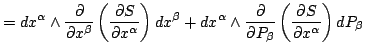
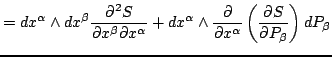
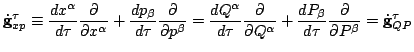
Discussion: Taking advantage of the chain rule, let

$$\mathbf{\dot{g}}^\tau_{xp}\equiv \frac{dx^\alpha}{d\tau} \frac{\p... ...{dP_\beta}{d\tau} \frac{\partial}{\partial P^\beta}=\mathbf{\dot{g}}^\tau_{QP}$$

be a vector tangent to the phasespace trajectory $\mathbf{g}^\tau$ relative to the given ( $x^\alpha;p_\beta$) and the new ( $Q^\alpha;P_\beta$) coordinates respectively.

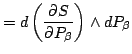
a) Show that

$$\langle dx^\alpha \wedge dp_\alpha \vert\mathbf{\dot{g}}^\tau_{xp}\rangle = dp_\alpha \frac{dx^\alpha}{d\tau}-dx^\beta \frac{dp_\beta}{d\tau}\langle dQ^\alpha \wedge dP_\alpha \vert\mathbf{\dot{g}}^\tau_{QP}\rangle = dP_\alpha \frac{dQ^\alpha}{d\tau}-dQ^\beta \frac{dP_\beta}{d\tau}$$ (9)

b) Point out why

$$\langle dx^\alpha \wedge dp_\alpha \vert\mathbf{\dot{g}}^\tau_{xp... ...e= \langle dQ^\alpha \wedge dP_\alpha \vert\mathbf{\dot{g}}^\tau_{QP}\rangle~.$$

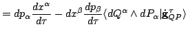
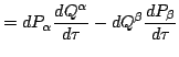
c) Show that

$$\langle dx^\alpha \wedge dp_\alpha \vert\mathbf{\dot{g}}^\tau_{xp}\rangle= d\mathcal{H}(x^\alpha,p_\beta)$$

implies Hamilton's equations of motion, Eq.(3)-(4).

d) Show that the introduction of the new coordinates $\{Q^\alpha,P_\alpha\}$ into $d\mathcal{H}$,

$$d\mathcal{H}(x^\alpha(Q^\gamma,P_\delta),p_\beta(Q^\gamma,P_\delta)) \equiv dH(Q^\gamma,P_\delta)$$

yields Eq.(6), Hamilton's equations relative to the new coordinates $\{Q^\gamma,P_\delta\}$.