


Next: Multipole Radiation Field
Up: Full Scalar Radiation Field
Previous: Full Scalar Radiation Field
The circumstance of long wave lengths is expressed by the inequality
where  is the radius of the cylinder surrounding the source. This
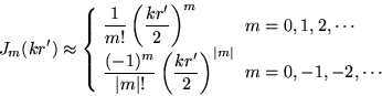
circumstance allows us to set
is the radius of the cylinder surrounding the source. This
circumstance allows us to set
 |
(46) |
throughout the integration region where the source is non-zero, and it
allows us to introduce the  st multipole moment (per unit length
 )
)
![\begin{displaymath}
\frac{i^m}{\vert m\vert !}
\int_0^\infty r'dr' \int_0^{2\pi}...
...rm{length}}
\times(\textrm{length})^{\vert m\vert +1}\right]
\end{displaymath}](img229.png) |
(47) |
for the double integral on the right hand side of Eq.(45). This multipole density [#!factor_of_two!#] is complex. However, the reality of the master source
 implies and is implied by
In terms of this multipole density the full scalar radiation field in  is
is
 |
| |
|
 |
(48) |
The evaluation of the mode integral
 is now
an easy two step task. First recall the
is now
an easy two step task. First recall the  th recursion relation
![\begin{displaymath}
e^{im\theta} J_m(kr)= \frac{(-1)^m}{k^{\vert m\vert}}
\left...
...l \theta} \right) \right]^m
J_0(kr),\quad m=0,\pm1,\pm2,\cdots
\end{displaymath}](img235.png) |
(49) |
where for negative one uses
This recursion relation is a consequence of consolidating two familiar
contiguity relations for the Bessel functions. Introduce Eq.(49) into the integrand of Eq.(48).
Second, use the standard expression
for the Dirac delta function. Apply this equation to
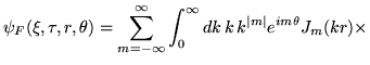
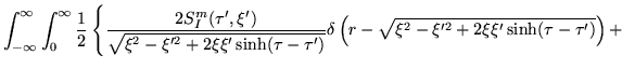
Eq.(48). Consequently, the full scalar
radiation field in Rindler sector reduces to the following
multipole expansion
![$\displaystyle \psi_F(\xi,\tau,r,\theta)= \sum_{m=-\infty}^\infty
(-1)^m \left[ ...
...tial \theta} \right) \right]^m \psi_m(\xi,\tau,r) \quad
\quad [\textrm{charge}]$](img238.png) |
|
|
(50) |
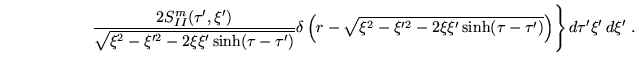
where
Doing the  -integration yields
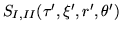
Here ![$[~~]_I$](img245.png) and
and ![$[~~]_{II}$](img246.png) mean that the source functions are
evaluated in compliance with the Dirac delta functions at
mean that the source functions are
evaluated in compliance with the Dirac delta functions at
 and
and
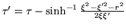 respectively. Recall
that is a strictly timelike coordinate in Rindler sector
respectively. Recall
that is a strictly timelike coordinate in Rindler sector  ,
while in the coordinate
,
while in the coordinate  is strictly spacelike. Consequently, one should not be
tempted to identify and with what in a static
inertial frame corresponds to evaluations at advanced or retarded
times. Instead, one should think of the observation event
is strictly spacelike. Consequently, one should not be
tempted to identify and with what in a static
inertial frame corresponds to evaluations at advanced or retarded
times. Instead, one should think of the observation event
 in and the source event
 in
as lying on each other's light cones
in
as lying on each other's light cones
both of which cut across the future event horizons
 of and
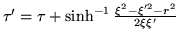
 . More explicitly, one has
which means that the source
 has been evaluated on
the past light cone
has been evaluated on
the past light cone
of at
 in Rindler
sector . Similarly,
in Rindler
sector . Similarly,
which means that the source
 has been evaluated on
the past light cone
has been evaluated on
the past light cone
of at
in Rindler sector . The
expression, Eq.(51), for the full
scalar radiation field is exact within the context of wavelengths
large compared to the size of the source. Furthermore, one should note
that even though there is only one  -integral,
  and
and
 are source functions with distinct domains, namely, Rindler
sectors and respectively.
are source functions with distinct domains, namely, Rindler
sectors and respectively.
Next: Multipole Radiation Field
Up: Full Scalar Radiation Field
Previous: Full Scalar Radiation Field
Ulrich Gerlach
2001-10-09
![$\displaystyle 2\int_0^\infty
\frac{\left[S^m_I(\tau',\xi')\right]_I -
\left[S^m...
...tau',\xi')\right]_{II}}{\sqrt{(\xi^2-\xi'^2-r^2)^2+(2\xi\xi')^2 }}
\xi' d\xi'~.$](img244.png)