


Next: Electric Dipole and its
Up: Axially Symmetric Source and
Previous: Axially Symmetric Source and
Consider radiation emitted from two magnetic dipoles. Have them be two
circular loop antennas each of area of  aligned parallel to
the
aligned parallel to
the  -plane with center on the
  -axis. Fix their location in
Rindler sectors
-axis. Fix their location in
Rindler sectors  and
and  by having them located at
  and
and
 so that they are accelerated into opposite
directions. Suppose each antenna has proper current
so that they are accelerated into opposite
directions. Suppose each antenna has proper current
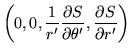
Then its magnetic moment is
its charge-flux four-vector obtained from Eq.(29) is
and the corresponding scalar source function  for Eq.(27) is
![\begin{displaymath}
S:\quad S_{I,II}(\tau',\xi',r',\theta')=
\frac{d~q_{I,II}(...
...uad \left[\frac{\textrm{charge}}{\textrm{length}^2}
\right]~.
\end{displaymath}](img324.png) |
(60) |
Here  is the Heaviside unit step function. The proper magnetic
dipole is the proper volume integral of this source,
is the Heaviside unit step function. The proper magnetic
dipole is the proper volume integral of this source,
Being symmetric around its axis, such a source produces only radiation
which is independent of the polar angle  . Consequently, all
partial derivatives w.r.t. vanish, and the full scalar field,
Eq.(54), in
. Consequently, all
partial derivatives w.r.t. vanish, and the full scalar field,
Eq.(54), in  becomes with the help of Eq.(47)
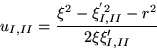
where
This is the T.E. scalar field due to a localized pair of axially symmetric
loop antennas, each one with its own time dependent current. By
setting one of them to zero one obtains the radiation field due to the
other.
Next: Electric Dipole and its
Up: Axially Symmetric Source and
Previous: Axially Symmetric Source and
Ulrich Gerlach
2001-10-09
![$\displaystyle i_{I,II}(\tau')\delta(\xi'-\xi'_{I,II})
\delta(r' -a)
\left(0,0,0...
...)~,\quad\quad\quad\quad
\left[\frac{\textrm{charge}}{\textrm{length}^3} \right]$](img323.png)
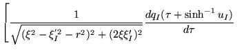
![$\displaystyle \left. \frac{1}{\sqrt{(\xi^2-\xi^{'2}_{II} -r^2)^2+(2\xi \xi'_{II...
...ac{dq_{II}(\tau-\sinh^{-1}u_{II})}{d\tau}
\right]~,\quad\quad [\textrm{charge}]$](img329.png)