Commensurable Accelerated Clocks

Again consider a pair of clocks AB and BC.

Figure 6: Two adjacent geometrical clocks consisting of collinearly accelerated cavities AB and BC, each containing a pulse bouncing back and forth. Depicted in this diagram is a sequence of 4 pulses coming from A and impinging on B which are matched by a sequence of 8 pulses coming from C. The ratio $c/a=8/4$ is the ticking rate of BC normalized to that of AB. The fact that this ratio stays constant throughout the history of the two clocks makes them also commensurable, just like those in Figure 5

But this time have all three of their radar units accelerate collinearly to the right with respective constant accelerations $1/\xi_A$, $1/\xi_B$, and $1/\xi_C$ respectively, and with common future and past event horizons, as in Figure 6. To make the discussion concrete, assume that $0<\xi_A <\xi_B <\xi_C$.

Consider the ticking produced by a pulse bouncing back and forth in clock AB. The proper time between two successive ticks at A is

$$\begin{eqnarray*} \xi_A \times \left(\begin{array}{c} \textrm{boost coordinate}... ... ticks} \end{array} \right) = \xi_A \times 2\log(\xi_B/\xi_A)~, \end{eqnarray*}$$

while at B it is

$$\begin{eqnarray*} \xi_B \times \left(\begin{array}{c} \textrm{boost coordinate}... ... ticks} \end{array} \right) = \xi_B \times 2\log(\xi_B/\xi_A)~, \end{eqnarray*}$$

Their ratio

$$\frac{2\,\xi_B \log(\xi_B/\xi_A)}{2\,\xi_A \log(\xi_B/\xi_A)}= \frac{\xi_B}{\xi_A}\equiv k_{AB}$$ (6)

is the pseudo-gravitational frequency shift factor. Similarly, for clock BC one has

$$\frac{\xi_C}{\xi_B}\equiv k_{BC}~.$$ (7)

These two frequency shift factors control the rate at which pulses arrive at B from A and C respectively. In fact, the two corresponding matched pulse sequences are

$$0,2\,\xi_B \log(\xi_B/\xi_A),\cdots,2\,a\xi_B \log(\xi_B/\xi_A)$$

and

$$0,2\,\xi_B \log(\xi_C/\xi_B),\cdots,2\,c\xi_B \log(\xi_C/\xi_B)~,$$

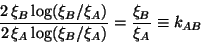
where the last pulse arrival time is the same, i.e.

$$2\,a\xi_B \log(\xi_B/\xi_A)=2\,c\xi_B \log(\xi_C/\xi_B)~,$$

or with the help of Eqs.(7) and (8)

$$\frac{c}{a}= \frac{(1/\log k_{BC})}{(1/\log k_{AB})}~.$$ (8)

This is the ticking rate of clock BC normalized relative to clock AB. This ticking rate is a constant independent of the starting time of the two matched pulse sequences. Consequently, accelerated clocks AB and BC are also commensurable.