Phase Flow: Its Trajectories and Transformations

Together with the spacetime gradient of $S$, Eqs.(15)-(19), the constructive interference conditions, Eq.(23), also yields a moving point in phase space. The starting point is $\{ Q^\alpha;P_\beta\}$ when $\tau=\tau_0$. When $\tau=\tau$ the point has reached $\{x^\alpha;p_\beta\}$. This moving point forms a trajectory in phase space,

$$\{x^\alpha(\tau);p_\beta(\tau):\alpha,\beta=0,1,2,3\}= \{u,v,x,y;p_u,p_v,p_x,p_y\}.$$

It is a solution to Hamilton's equations of motion, Eqs.(3)-(4).

Problem 4: Show that (a) the conditions for constructive interference, Eq.(23), together with (b) the fact that the dynamical phase $S(x^\alpha;P_\beta)$ satisfies the H-J equation, Eq.(12), imply that each phase trajectory satisfies the Hamiltonian equations of motion, Eqs.(3) and (4).

Hint: Differentiate the H-J equation

$$\mathcal{H}\left( x^\alpha(\tau), \frac{\partial S(x^\gamma(\tau)... ...lpha}\right) + \frac{\partial S(x^\gamma(\tau),P_\beta;\tau)}{\partial \tau}=0$$

with respect to each of the constants of motion $P_\beta$. Differentiate the four equations for constructive interference

$$\frac{\partial S(x^\gamma(\tau),P_\beta;\tau)}{\partial P_\beta}=0$$

with respect to the world line parameter $\tau$. Compare the results. Next differentiate the H-J equation with respect to each of the coordinates $x^\alpha$.

Consider the set of phase space trajectories obtained from the dynamical phase $S$. For fixed $\tau$ they yield the map

$$\boxed{ \begin{array}{rcl} \mathbb{R}^8 &\stackrel{\displaystyle\... ...}^\tau(Q^\alpha;P_\beta)\equiv \{x^\alpha(\tau);p_\beta(\tau)\}~, \end{array} }$$ (27)

where, according to Eqs.(16)-(18) and (24)-(27),

$$\{x^\alpha,p_\alpha \}= (u,v,x,y;p_u,p_v,p_x,p_y).$$

The relation $\mathbf{g}$ is called the phase flow generated by the superhamiltonian $\mathcal{H}$. Physically this flow expresses the evolution of a collisionless ensemble of charged particles each launched with its own $(Q^\alpha,P_\beta)$ in the field of a laser. Mathematically this flow combines two concepts into one: letting $\tau$ vary while keeping $\{ Q^\alpha;P_\beta\}$ fixed yields a phase space trajectory; letting $\{ Q^\alpha;P_\beta\}$ vary while keeping $\tau$ fixed yields a (canonical) transformation, Eq.(28). Combining the two, one obtains $\mathbf{g}^\tau$, a $\tau$-parametrized family of transformations which expresses the nonintersecting trajectories of a set of moving points, each one labelled by eight coordinates.

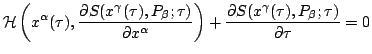
The geometrical representation of these transformations is depicted in Figure 8: Points of the intersection of the straight trajectories with a $(Q^\alpha;P_\beta)$-plane in (b) get mapped into the intersection of the curved trajectories with a $(q^\alpha;p_\beta)$-plane in (a).

Figure 8: Three trajectories in the extended phase space relative to (a) the given physical coordinates $\{x^\alpha ,p_\beta ,\tau -\tau _0\}\equiv (u,v,x,y;p_u,p_v,p_x,p_y,\tau -\tau _0)$ and (b) the new coordinates $\{Q^\alpha ,P_\beta ,\tau -\tau _0\}\equiv (Q^\tau ,Q^v,Q^x,Q^y;P_\tau ,P_v,P_x,P_y,\tau -\tau _0)$ relative to which the trajectories are straight lines. The mapping $\mathbf{g}$ is the phase flow map discussed in the text.

Consider the transformation corresponding to $\tau=\tau_1$,

$$\mathbf{g}^{\tau_1}(Q^\alpha;P_\beta)=\{Q_1^\alpha;P_{1\beta}\}~.$$ (28)

Then

$$\mathbf{g}^\tau(Q_1^\alpha;P_{1\beta})=\mathbf{g}^\tau\circ \mathbf{g}^{\tau_1}(Q^\alpha;P_\beta)$$ (29)

is the composite of $\mathbf{g}^\tau$ and $\mathbf{g}^{\tau_1}$. But both $\mathbf{g}^\tau\circ \mathbf{g}^{\tau_1}(Q^\alpha;P_\beta)$ and $\mathbf{g}^{\tau+\tau_1}(Q^\alpha;P_\beta)$ are solutions to the same (time-independent!) Hamilton's equations of motion with the same starting point. Consequently,

$$\mathbf{g}^\tau\circ \mathbf{g}^{\tau_1}(Q^\alpha;P_\beta))= \mathbf{g}^{\tau+\tau_1}(Q^\alpha;P_\beta)$$

One sees that $\mathbf{g}^{\tau=0}$ is the identity map, and $\mathbf{g}^{-\tau}={(\mathbf{g}^{\tau})}^{-1}$ is the inverse map. Consequently, Eq.(28) is a $\tau$-parametrized group of phase space coordinate transformations, the phase flow of $\mathcal{H}$. Being generated by the dynamical phase $S$, they are canonical transformations whose defining property is Eq.(8).

These transformations have a striking simplifying effect on the phase space trajectories. Suppose one considers the extended phase space,

$$\mathbb{R}^9=\mathbb{R}^8\times \mathbb{R}~~\textrm{where}~\mathbb{R}=\tau\textrm{-axis}$$

It is (8+1)-dimensional and it is obtained from $\mathbb{R}^8$ by adding the $\tau$-line as an extra coordinate axis. In this space the phase space trajectories are represented by curved non-intersecting lines as in Figure 8(a). The $\tau$-parametrized canonical transformation constitute a map from a $(x^\alpha;p_\beta,\tau)$-coordinatized copy of the extended phase space $\mathbb{R}^9$ to a $(Q^\alpha;P_\beta,\tau)$-coordinatized copy of the same extended phase space $\mathbb{R}^9$. The benefit of the latter is that relative to it the phase space trajectories are straightened out as in Figure 8(b).

However, as intimated by Eq.(23), the same constructive interference conditions also imply a $\tau$-dependent canonical coordinate transformation,

$${ \{Q^\alpha,P_\alpha\}\equiv (Q^\tau,Q^v,Q^x,Q^y;P_\tau,P_v,P_x,,P_y) \stackrel{\displaystyle\mathbf{g}^\tau}{\rightsquigarrow } }$$

$$~~~~~~~~~~~~~~~~~~~\{x^\alpha,p_\alpha \}\equiv (u,v,x,y;p_u,p_v,p_x,y,p_y)$$

This transformation, which is given (implicitly) by Eqs.(19)-(18) and (25)-(27), is generated by the Hamilton-Jacobi function, Eq.(20). This transformation straightens out the phase space trajectories (as depicted in Figure 8) of Hamilton's equations of motion (3) and (4).

Problem 5: Write down and solve Hamilton's equations of motion, (3)-(4), and verify that the solution coincides with the constuctive interference condition, Eqs.(24)-(27)