Next: Frequency of Rotation
Up: Action Variables
Previous: Canonical Transformation
Contents
3. Each of the four coordinates, Eq.(![[*]](crossref.png) ), is the angular coordinate on one of the circles
which makes up the torus, Eq.(34). Furthermore, the
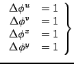
periodicity of each is measured in units of revolutions, one per period:
), is the angular coordinate on one of the circles
which makes up the torus, Eq.(34). Furthermore, the
periodicity of each is measured in units of revolutions, one per period:
The existence and the magnitude of four periods expressed by these
equations is validated by the ensuing calculation. One takes
advantage of the four-fold periodicity of the spacetime environment
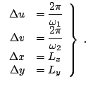
of the particle's world line. This periodicity is characterized by the
four periods
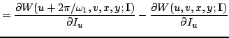
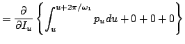
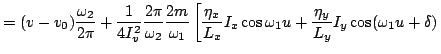
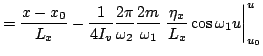
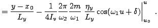
The transformation, Eq.(52), maps the
given spacetime periods, Eq.(55), into the
periods, Eq.(54), of the torus. For
example, using Eqs.(52) and
(42) one has
Analogous computations validate the remaining periodicities in
Eq.(54).
For fixed action
 the periodic angle
coordinates
the periodic angle
coordinates
 span a
four-dimensional torus, Eq.(34), while a given spacetime
trajectory, Eqs.(48)-(51), is represented by a straight line winding on
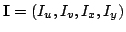
it. The relation between these toroidal coordinates and the physically
given ones is
span a
four-dimensional torus, Eq.(34), while a given spacetime
trajectory, Eqs.(48)-(51), is represented by a straight line winding on
it. The relation between these toroidal coordinates and the physically
given ones is
In the framework of this toroidal picture the physical coordinates
are curvilinear, but the geometrical coordinates are rectilinear.
Because of their geometrical simplicity, the action-angle
variables are sometimes called normal coordinates.
Next: Frequency of Rotation
Up: Action Variables
Previous: Canonical Transformation
Contents
Ulrich Gerlach
2005-11-07