Next: Linear Representation
Up: Action-Angle Representation
Previous: Multiple Periodicity expressed in
Contents
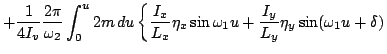
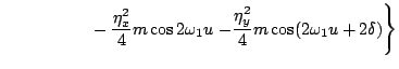
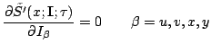
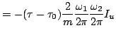
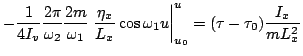
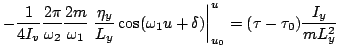
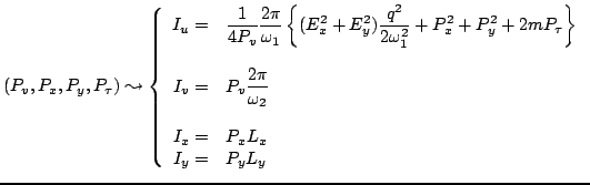
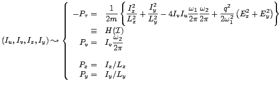
The four periods give rise to the four action variables
The evaluation of these integrals is done with the help of
Eqs.(16)-(18) and (31)-(32). The result is the transformation
and its inverse
The effect of this transformation is that it decomposes the dynamical
system into its fundamental physical - and hence mathematical - components,
each having its own frequency.
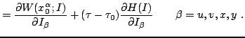
Indeed, introducing the action variables into the dynamical phase,
Eq.(22), one finds that, with the help
of Eqs.(31) and (32), its form (a.k.a. ``Hamilton's
principal function'') is
 |
(40) |
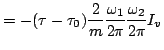
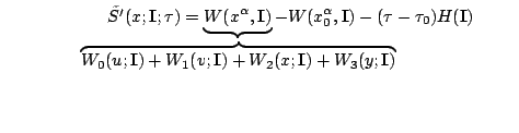
where the four contributions to Hamilton's characteristic function
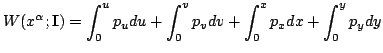 |
(41) |
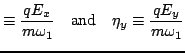
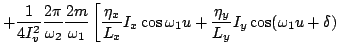
are
as the dimensionless relativistic impulse factors, which express
the interaction between the laser and the charge,
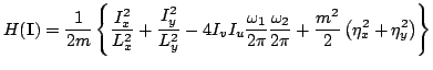
while
is the conserved superhamiltonian,
Eq.(40), expressed in terms of the
four action variables.
The introduction of these variables into the dynamical phase, and their
application to the principle of constructive interference,
again leads to a straightening out of the phase space trajectories,
just like Eq.(23) led to Figure
8b. The only difference is that now
the straight lines are tilted relative to the coordinate plane
 . This means that the straight lines have nonzero
projections onto this plane.
These projected paths are
. This means that the straight lines have nonzero
projections onto this plane.
These projected paths are
They lead to a number of conclusions.
- Problem6: a) Point out why these four equations express the
same spacetime trajectory as Eqs.(23).
b) show that their explicit form is
Subsections
Next: Linear Representation
Up: Action-Angle Representation
Previous: Multiple Periodicity expressed in
Contents
Ulrich Gerlach
2005-11-07