Tropical Geometry of genus two curves

Web page for the paper by María Angélica Cueto and Hannah Markwig

The computational results in this web page were obtained using the software packages SAGE 6.9, Macaulay 2, and Singular, including the special library tropical.lib. The sage outputs are stored as .sobj files and plain text files (as commends in the scripts). The Macaulay 2 outputs are recorded as comments on the scripts.

All scripts and outputs described in this page are available as a zip file here. CAVEAT: Some of the .sobj files may not load when working with earlier versions of SAGE. You can run the scripts to obtained readable .sobj files.

Jump to:

Naive tropicalization of plane hyperelliptic curves and tropical modifications inducing faithful tropicalizations

Igusa invariants and their tropicalizations

§0. Naive tropicalization of plane hyperelliptic curves and tropical modifications inducing faithful tropicalizations

The following scripts allow us to produce faithful tropicalizations on the minimal skeleton (or extended, whenever indicated) of all genus 2 smooth curves defined over a non-Archimedean field K with a valuation val: K^* → R. Our input data for the curve is the hyperelliptic equation, i.e. its six ramification points α₁,…,α₆ in P¹. Furthermore, we may assume α₁= (0,1) and α₆=(0,1) (with -val(α₁)="-Infinity", -val(α₁)="+Infinity"), and the remaining α₂,…,α₅ lie in K^*. Their negative valuations

ω_i = -val(α_i) for i = 2,…,5, d₃₄ = -val(α₃ - α₄)

and the initial forms in(α_i) satisfy the required conditions indicated in Table 1.

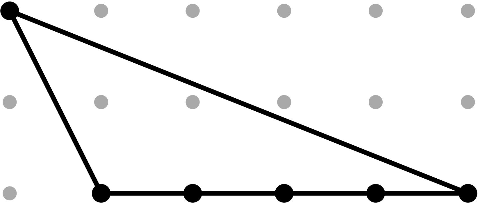
**Table 1: Classification of skeleta of smooth genus 2 curves.**
Cell	Extended skeleta	Defining conditions	Lengths
(I)		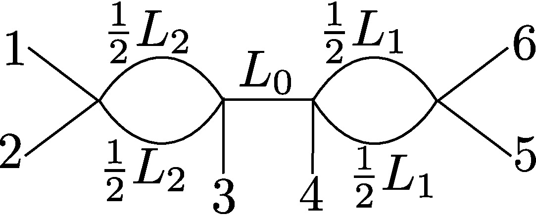ω₂ < ω₃ < ω₄ <ω₅	L₀ = (ω₄ - ω₃)/2 L₁ = 2(ω₅ - ω₄) L₂ = 2(ω₃ - ω₂)
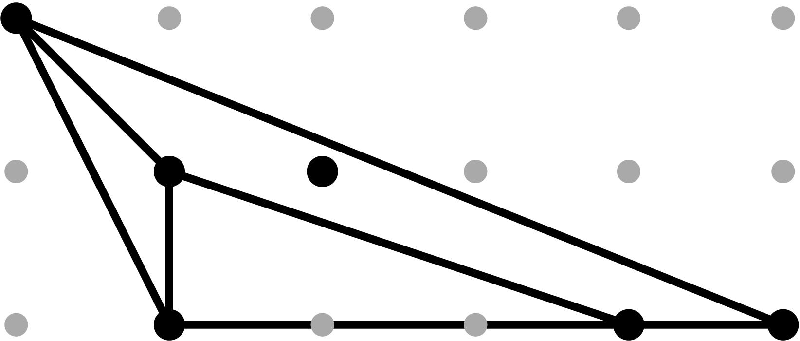
(II)		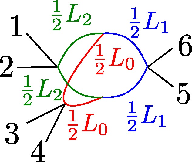ω₂ < ω₃ = ω₄ <ω₅ d₃₄<ω₃ in(α₃)=in(α₄)	L₀ = 2(ω₄ - d₃₄) L₁ = 2(ω₅ - ω₃) L₂ = 2(ω₃ - ω₂)
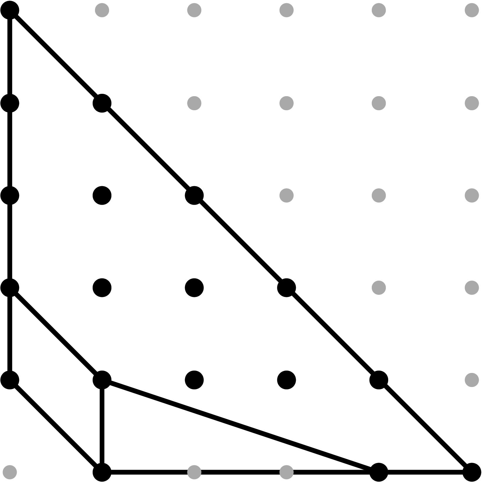
(III)		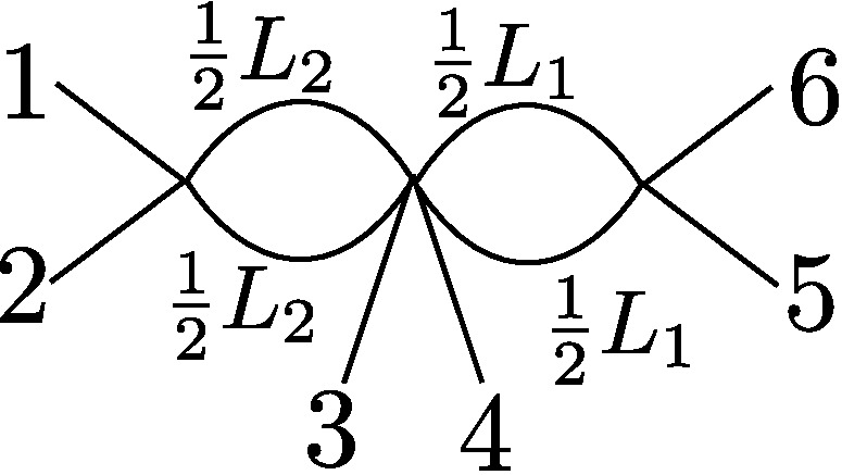ω₂ < ω₃ = ω₄ <ω₅ d₃₄ = ω₃ in(α₃) ≠ in(α₄)	L₀ = 0 L₁ = 2(ω₅ - ω₃) L₂ = 2(ω₃ - ω₂)
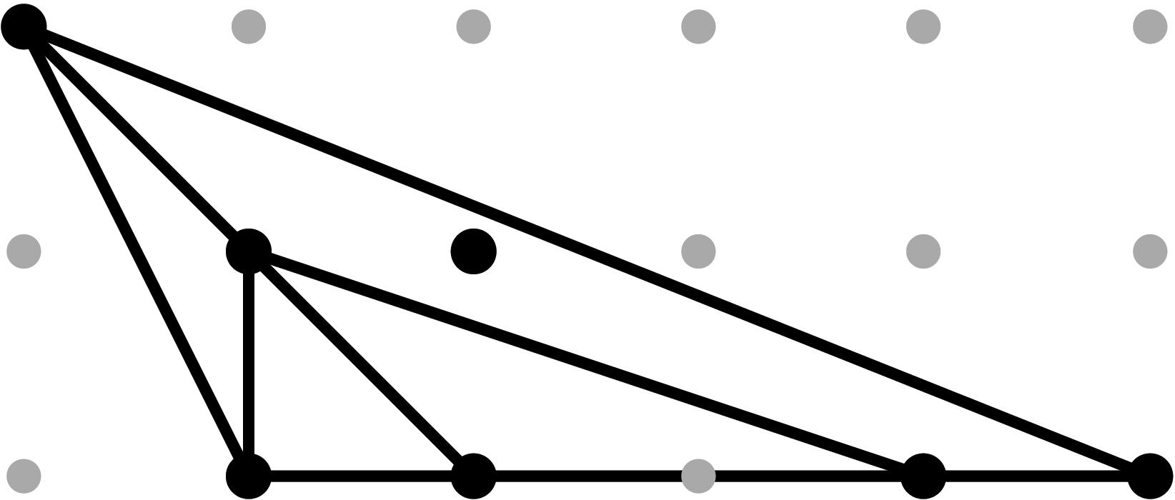
(IV)		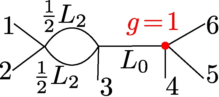ω₂ < ω₃ < ω₄ ω₄ = ω₅ in(α₄) ≠ in(α₅)	L₀ = (ω₄ - ω₃)/2 L₁ = 0 L₂ = 2(ω₃ - ω₂)
(V)		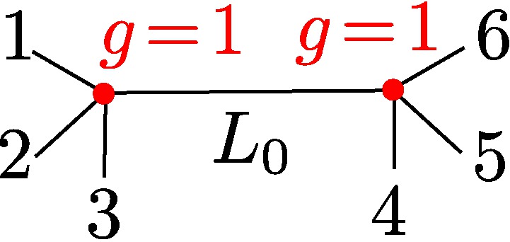ω₂ < ω₄ ω₂ = ω₃ ω₄ = ω₅ in(α₂) ≠ in(α₃) in(α₄) ≠ in(α₅)	L₀ = (ω₄ - ω₃)/2 L₁ = 0 L₂ = 0
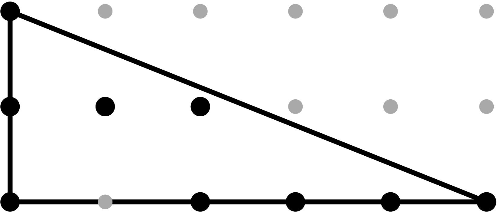
(VI)		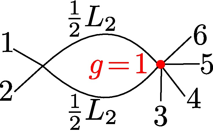ω₂ < ω₃ ω₃ = ω₄ = ω₅ in(α₃) ≠ in(α₄) in(α₃) ≠ in(α₅) in(α₄) ≠ in(α₅)	L₀ = 0 L₁ = 0 L₂ = 2(ω₃ - ω₂)
(VII)		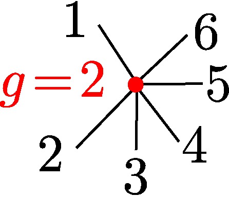ω₂ = ω₃ = ω₄ = ω₅ in(α_i) ≠ in(α_j) (for i≠ j)	L₀ = 0 L₁ = 0 L₂ = 0

The naive tropicalization induced by the hyperelliptic equation

g(x,y) = y² - x (x- α₂)(x- α₃)(x- α₄)(x- α₅)

is never faithful. We use the tropical modification of R² along the tropical polynomial

F(X,Y) = max{Y, A + X, B + 2X} for A = (ω₅ + ω₄ + ω₃) / 2 and B = ω₅ / 2.

A lifting of this tropical polynomial yields a faithful tropicalization on the minimal skeleta via the ideal I_g,f = ⟨ g(x,y), z-f(x,y) ⟩ ⊂ K[x^±, y^±, z^±], i.e. trop(f) = F where

f(x,y) = y - (- α₅ α₄ α₃)^1/2 x + ( - α₅)^1/2 x².

Since the lifting f(x,y) of the modification involves square roots of the branch points, we replace the 4 varying branch points α_i by squares of 4 new variables b_i, i.e.

α₂ = b₂² , α₃ = b₃² , α₄ = b₄² and α₅ = - b₅², so ω_i = - 2 val(b_i) for i = 2, 3, 4, 5 .

Therefore the hyperelliptic equation becomes

g(x,y) = y² - x (x - b₂²)(x - b₃²)(x - b₄²)(x + b₅²)

The combinatorial types of the tropical curves of Type II defined by the ideal I_g,f are determined by means of the Newton subdivisions of the 3 coordinate projections. In order to characterize them, we compute the coefficients of each of the 3 defining equations in terms of the parameters b₅, b₄, b₃, b₂ in Singular (in a second step we replace b₃ = b₄ + b₃₄. In all cases, the (x,y)-projection is well understood: it looks like the Type III case except that the x³ point is marked.

Sage script containing implementations of all the relevant functions for computing leading terms of polynomials with respect to a weight order, intersections of fans and cones, computation of rays of a cone and sample points in the relative interior of a cone (obtained as the sum of its extremal rays)
Singular script computing the coefficients of x², x³, and x⁴ of the equation defining the (x,z)-projection. The script outputs the corresponding 3 polynomials in b₅, b₄, b₃ and b₂. [Output in plain text] [Output that will be used by the relevant Sage script]
Singular script computing the coefficients of y⁴, y³z, y²z², yz³, z⁴, y³, y²z, yz², z³, y², yz, z², y, z of the equation defining the (y,z)-projection (the remaining coefficients are monomials in the variables b₅, b₄, b₃ and b₂, so their valuation is linear in the Type II Cone.) Caveat: the variables are labelled x and y instead of y and z in the script. The order of the monomials and labelling of the variables will be preserved throughout subsequent scripts. The script outputs the corresponding 14 polynomials in b₅, b₄, b₃ and b₂ [Output in plain text] [Output that will be used by the relevant Sage script]

Furthermore, if we add a tail (i.e., an element in K with valuation -A + ε and -B + ε', respectively, with 0<ε, ε'<<1) to the coefficients of f(x,y) we obtain a faithful tropicalization of the extended skeleta for types (I) and (III). We called such choice a "refined modification."

Singular script computing the coefficients of x², x³, x⁴, x²z and xz of the equation defining the (x,z)-projection with respect to the refined modification. The script outputs the corresponding polynomials in b₅, b₄, b₃ and b₂. [Output in plain text] [Output that will be used by the relevant Sage script]

In the following sections, we describe the resulting faithful tropical curve in R³ by means the three coordinate projections and the Newton subdivisions of the resulting plane curves. Numerical examples for K = Q[t] illustrate each of the various cases that arise. To simplify the expressions, all our branch points are (up to sign) squares of polynomials in t with integer coefficients.

We provide Singular scripts as well as the output tropical curve for each projection computed with the Singular library tropical.lib. Each Singular file contains the defining equations for each plane equation.

Whenever ω_i = ω_j for i ≠ j, the legs l_i, and l_j in the extended Berkovich skeleta of the curve X marked with the branch points α_i and α_j map to the same leg in the naive tropicalization. If k of them meet, we separate them by means of k-1 vertical modifications along max{X,ω_i₁} with liftings z_{i_j} = x - α_{i_j} for j=1, …, s-1.

In Types (IV) and (V) we show that each vertex in the xy- and yz-projections dual to a lattice triangle with a unique interior vertex is the image of the corresponding genus 1 vertex in the Berkovich skeleton. We do so by means of a j-invariant computation.

By truncating the input equation, we obtain a smooth elliptic curve E_v (supported on the triangle).
We use Singular to compute the j-invariant. We use SAGE and Macaulay 2 to analyze the expected valuation of both the numerator and denominator of each j-invariant in terms of the negative valuations of the branch points by means of a leading term computation with a random integer vector ω = (ω₂,ω₃,ω₄,ω₅) ∈R⁴ in the corresponding Type (IV) of (V) Cones.
In all cases we show that - val(j(E_v)) ≤ 0, so the corresponding elliptic curves have good reduction.
We show that the corresponding Type (IV) of (V) Cones lie in a single cone of the Gröbner fan of both the numerator and denominator of the corresponding j-invariant. So the computation is independent of the chosen weight vector ω.
Since the leading terms have coefficients that are powers of 2, the computation is valid for any characteristic of the residue field other than 2.

§0.1 Type (I) Cone (Dumbbell):

**Table 0.1: Dumbbell Graph Files and Projections.**
Branch points	Singular Scripts	(x,y)-subdivision	(x,z)-subdivision	(y,z)-subdivision
α₂ = (t¹⁰+t¹²)² α₃ = (t⁵+t⁹)² α₄ = (3 t³+t⁸)² α₅ = -(1+t⁵)²	Standard Script (no refinement)	tex output ps output	tex output ps output	tex output ps output
α₂ = (t¹⁰+t¹²)² α₃ = (t⁵+t⁹)² α₄ = (3 t³+t⁸)² α₅ = -(1+t⁵)²	Refinement Script (t^ε and t^ε') ε = 4 ε'= 2	tex output ps output	tex output ps output	tex output ps output

§0.2 Type (II) Cone (Theta Graph):

This is the most challenging cell from the combinatorics perspective, since its the only case for which the chart σ₄ contains points of the tropical curve in its relative interior. Assuming the initial terms of the branch points to be generic, there will be exactly eight combinatorial types for the modified tropical curve in R³, coming from a subdivision of the Type II Cone into three pieces, obtained by adding the sum of the three extremal rays, and subdividing the cone accordingly. More types will arise in the non-generic case. Our proof by explicit computation determines these conditions in a precise fashion. Examples for each case are provided in the tables below.

Since the lifting f(x,y) of the modification involves square roots of the branch points, we replace the 4 varying branch points α_i by squares of 4 new variables b_i for i = 2, 3, 4, 5. Furthermore, since the valuation of α₃ - α₄ is relevant in this cell, we will replace b₃ by introducing a new variable b₃₄ = b₃-b₄, i.e.

α₂ = b₂² , α₃ = (b₄ + b₃₄)² , α₄ = b₄² and α₅ = - b₅², so ω_i = - 2 val(b_i) for i = 2, 4, 5 and d₃₄ = - val(b₃₄) - val(b₄).

Therefore the hyperelliptic equation becomes

g(x,y) = y² - x (x - b₂²)(x - (b₄+b₃₄)²)(x - b₄²)(x + b₅²)

To avoid working with non-real expressions, we sometimes replace α₂ with - b₂² (it will be indicated accordingly). In the new coordinates

(v₅, v₄, v₃₄, v₂) := (-val(b₅), -val(b₄), -val(b₃₄), -val(b₂)).

the Type II Cone is defined by the following inequalities:

v₅ > v₄ , v₄ > v₃₄ , and v₄ > v₂.

We record the 17 relevant coefficients for the (x,z)- and (y,z)-projections in terms of the parameters b₅, b₄, b₃₄ and b₂:

Plain text file containing the coefficients of x², x³, and x⁴ of the equation defining the (x,z)-projection. The result was computed with this Sage script.
Plain text file containing the coefficients of y⁴, y³z, y²z², yz³, z⁴, y³, y²z, yz², z³, y², yz, z², y, z of the equation defining the (y,z)-projection (the remaining coefficients are monomials in the variables b₅, b₄, b₃₄ and b₂, so their valuation is linear in the Type II Cone.) The result was computed with this Sage script.

In order to find all possible combinatorial types of resulting modified 3D-tropical curves with Theta graphs as minimal skeletons, we must compute the Gröbner fans of all the relevant coefficients, to decide what is the height function for each corresponding lattice point in the Newton polytope of the defining equations.

Sage script that computes the Gröbner fan of all the 3 non-monomial coefficients of the (x,z)-projection and their common refinement. We record the combinatorics of each fan as commented code on the Sage script, and the output as a fan and a dictionary of maximal cones, both as Sage object files. [Compresent output, consisting of '.sobj' files].
Sage script that computes the Gröbner fan of all the 14 non-monomial coefficients of the (y,z)-projection and their common refinement. We record the combinatorics of each fan as commented code on the Sage script, and the output as a fan and a dictionary of maximal cones, both as Sage object files. [Compresent output, consisting of .sobj files]
Sage script that computes the Gröbner fan of the product of all relevant 17 non-monomial coefficients of the (x,z) and (y,z)-projection. The resulting fan as f-vector [1, 21, 54, 35] and lineality space spanned by the all-ones vector.
Sage object: common refinement of all 17 Gröbner fans, encoded as a polyhedral fan data-type in Sage.
Sage object: dictionary of all 35 maximal cones in the common refinement of all 17 Gröbner fans (with keys given by numbers 0 through 34).

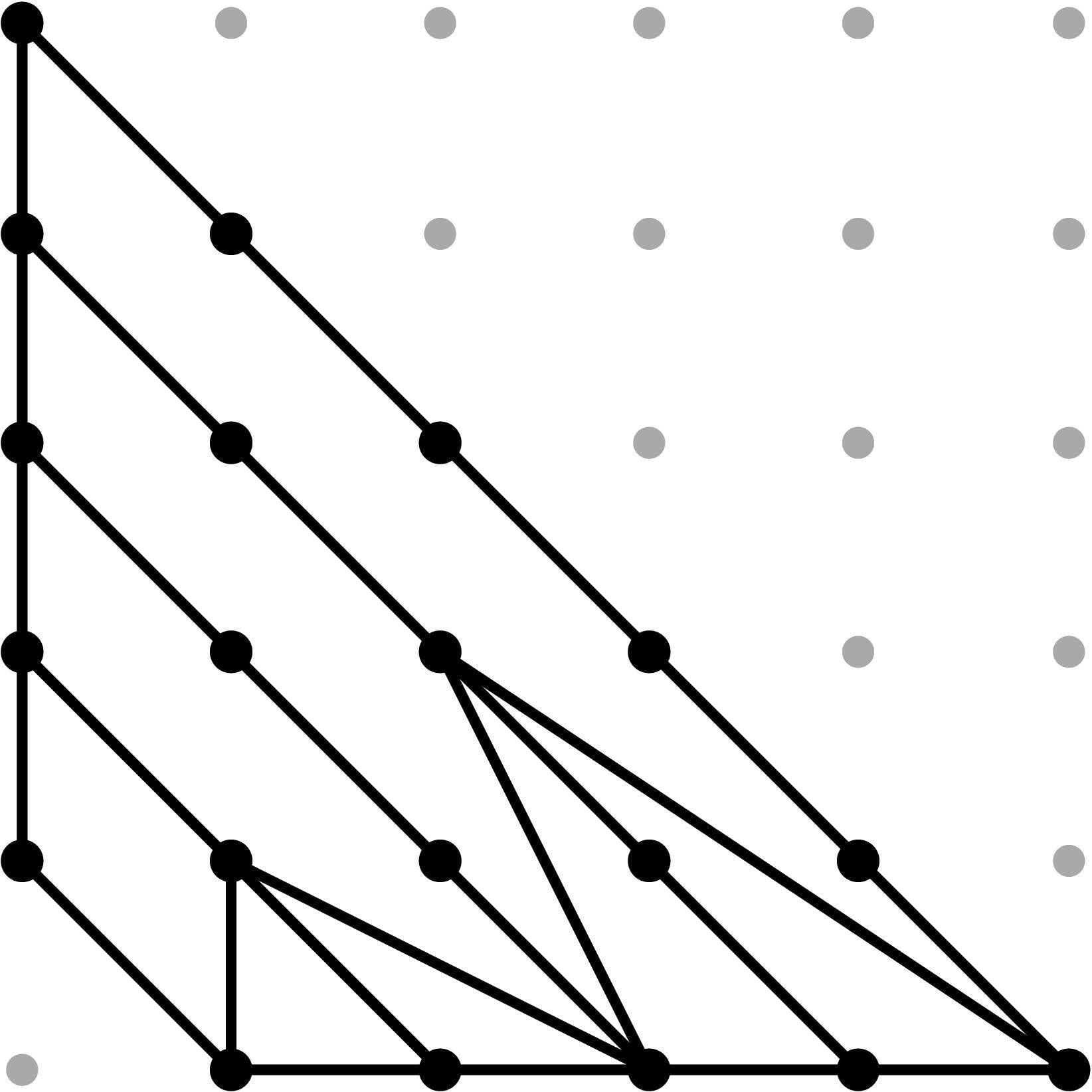
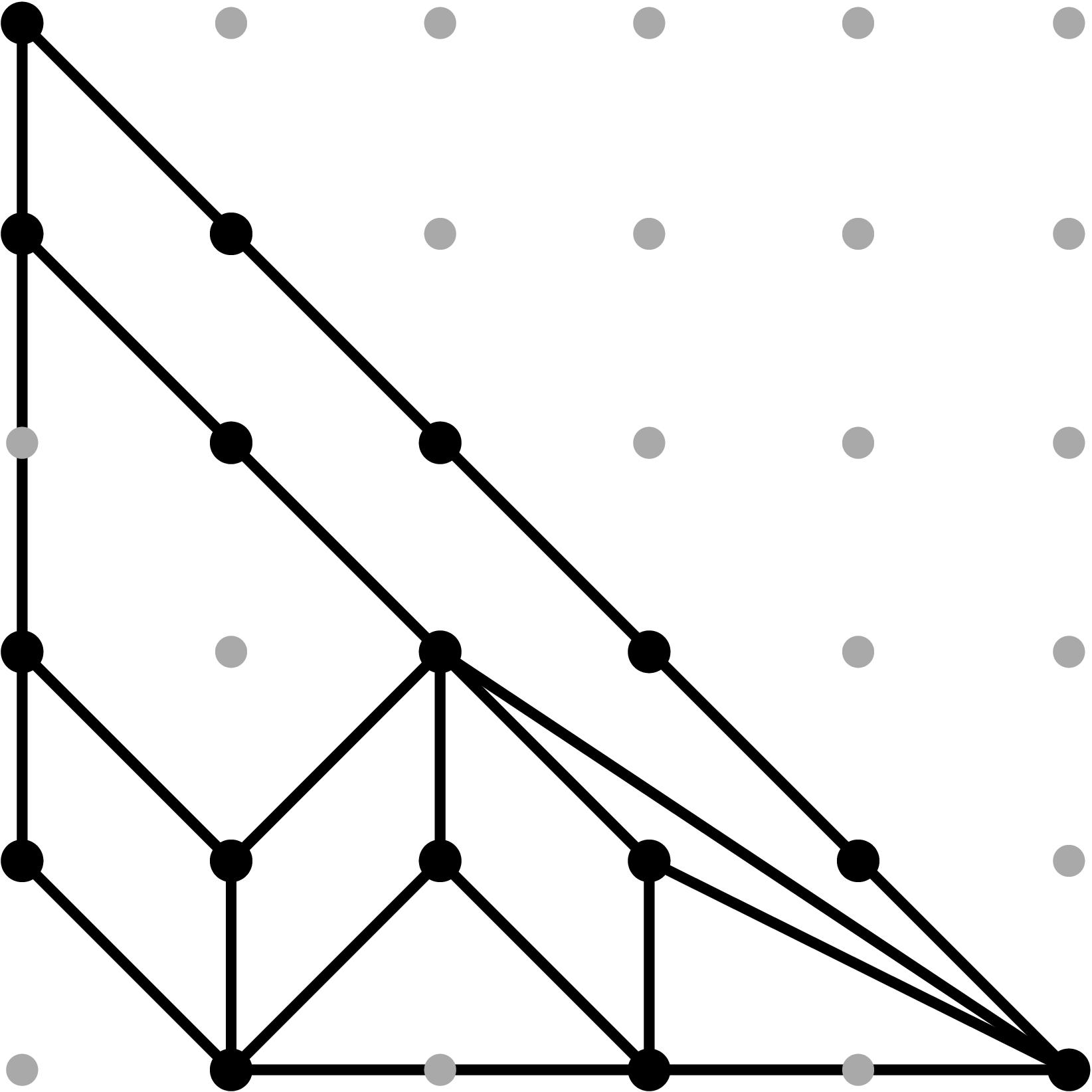
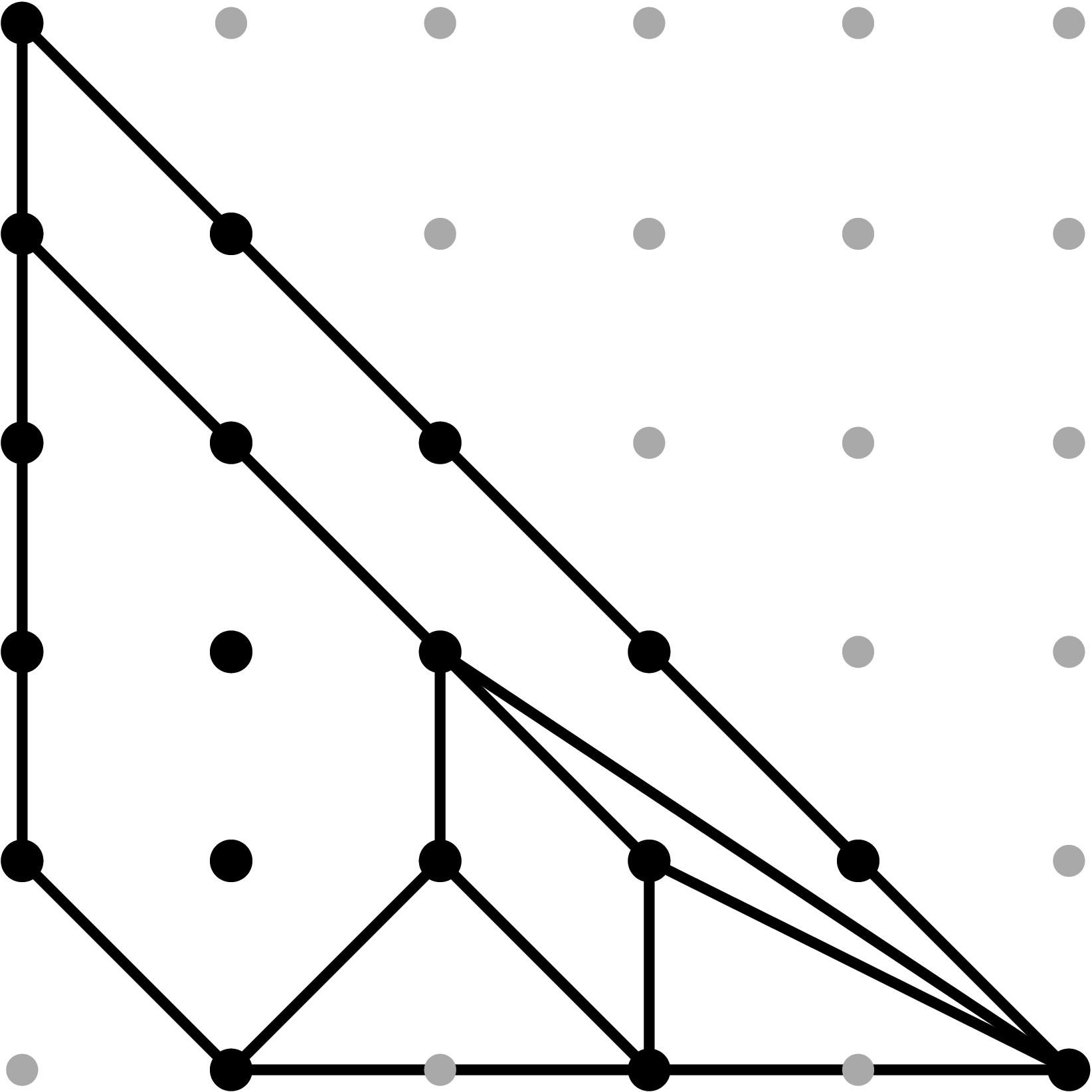
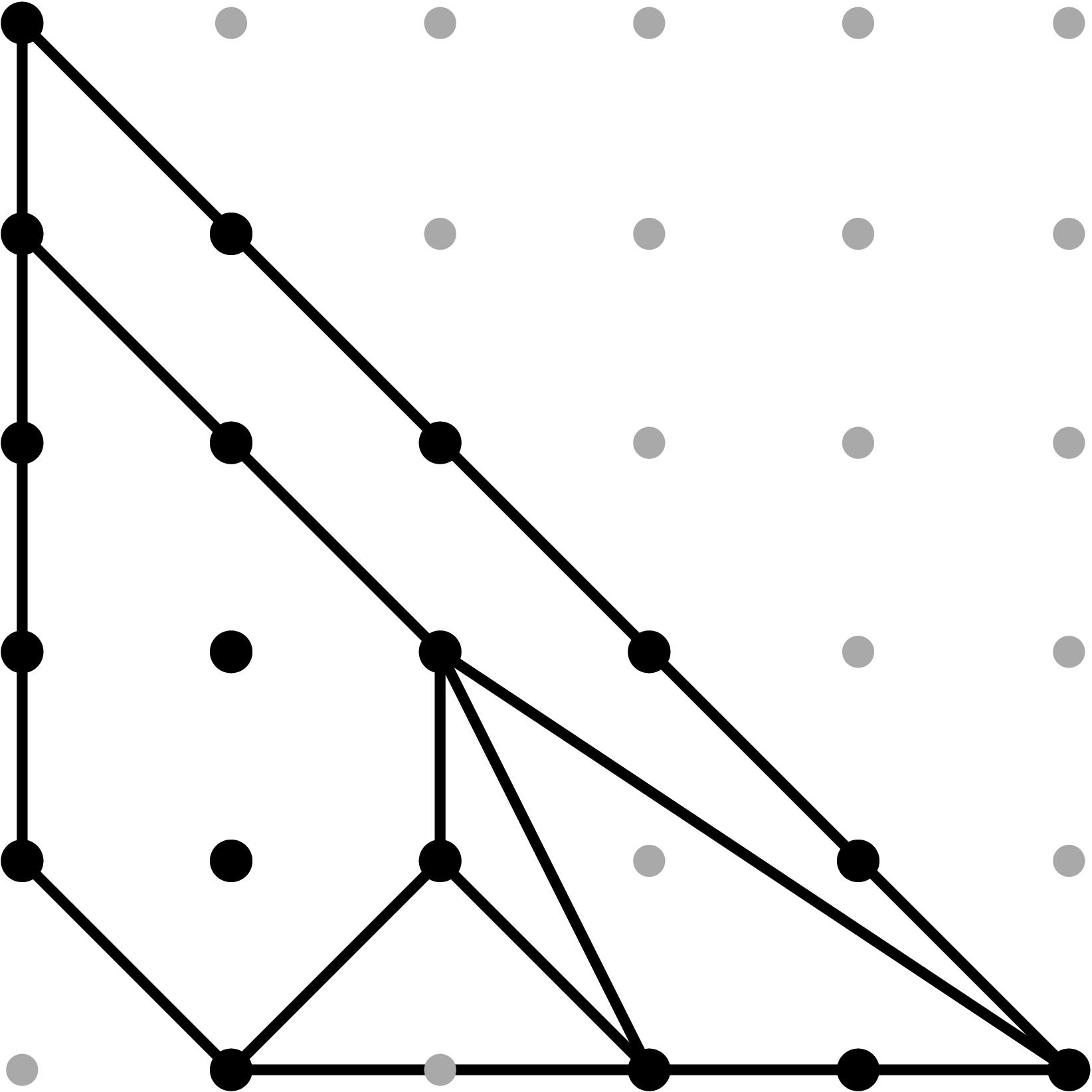
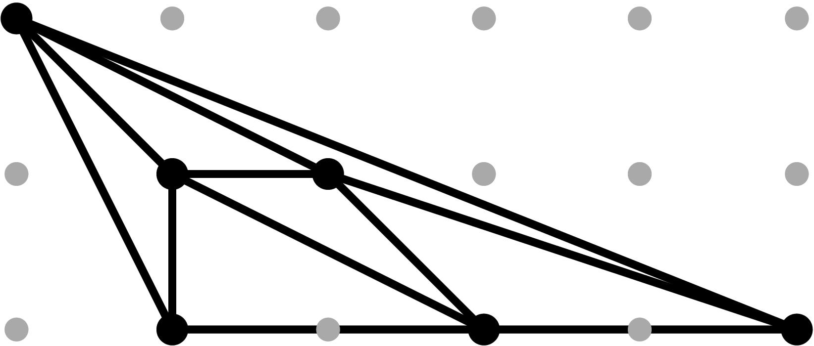
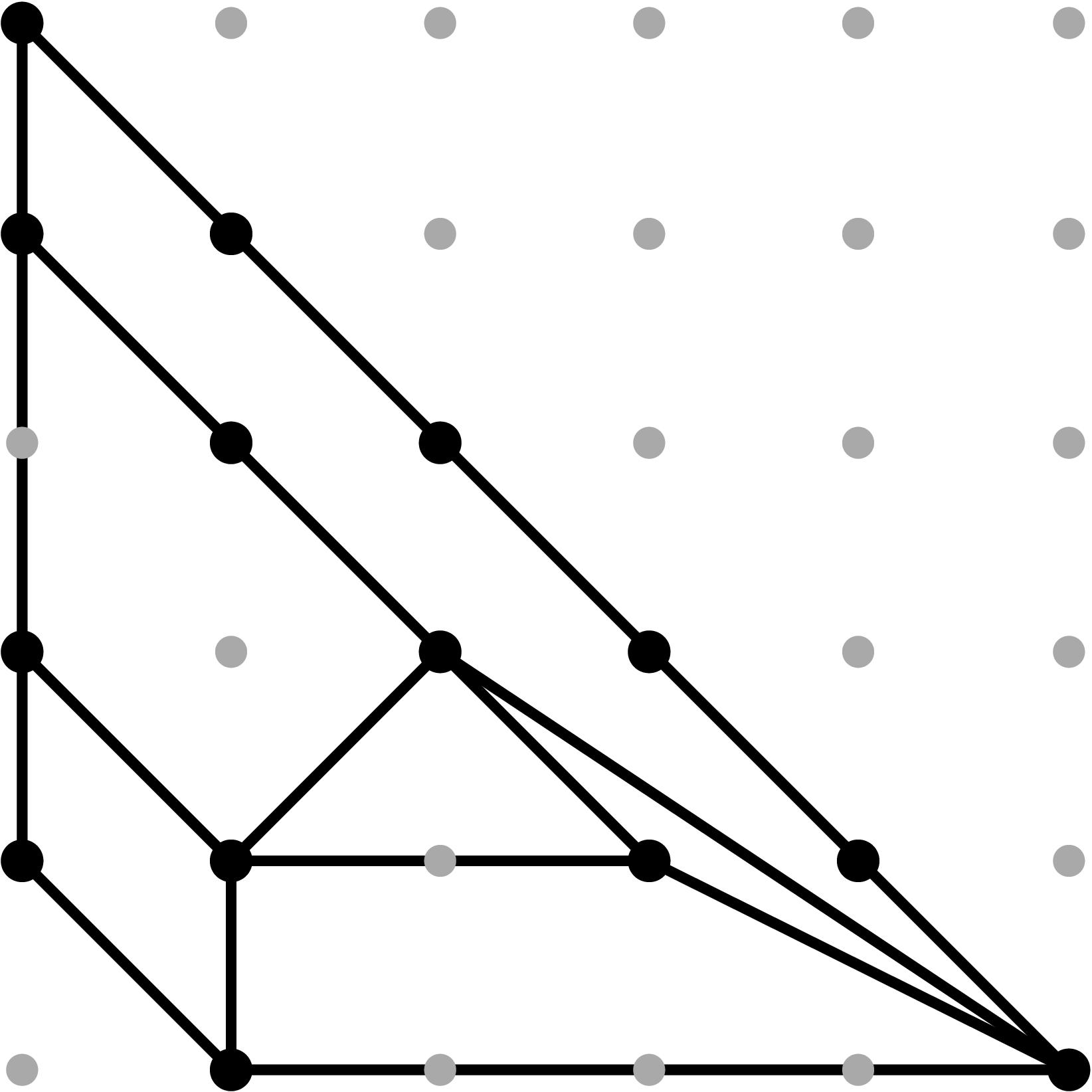
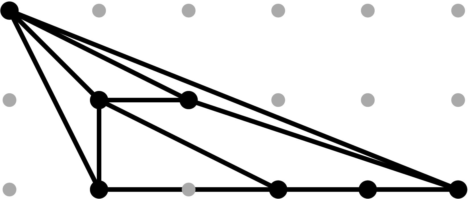
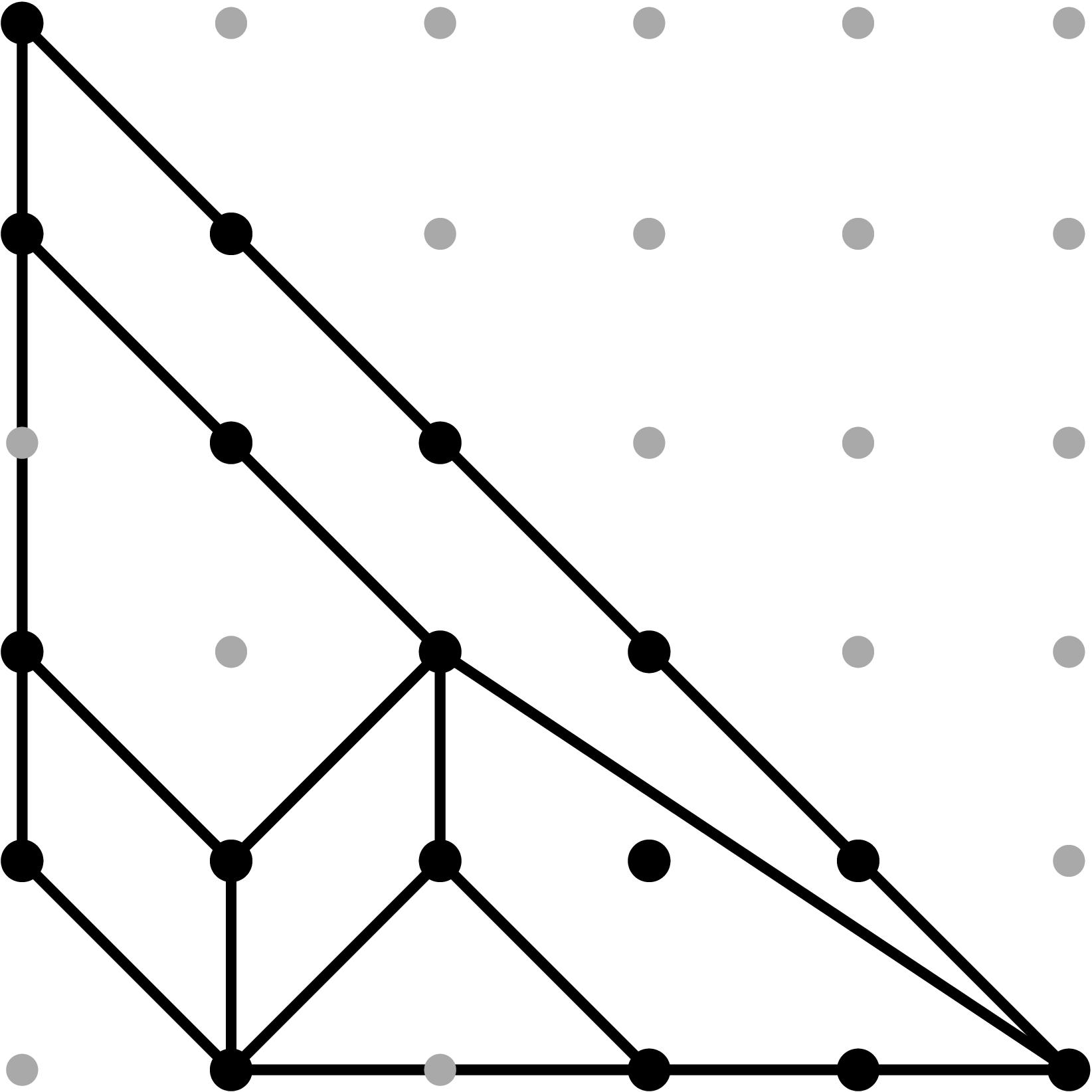
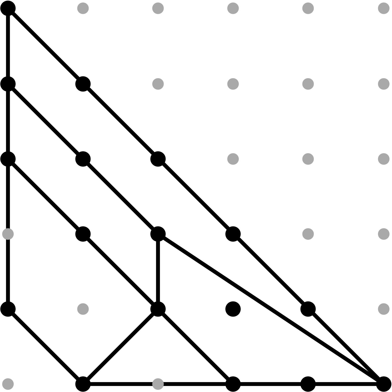
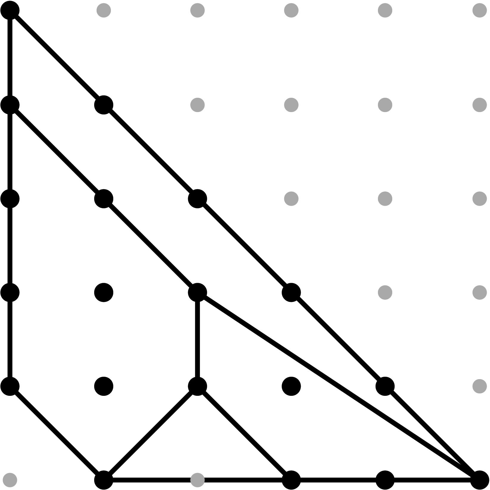
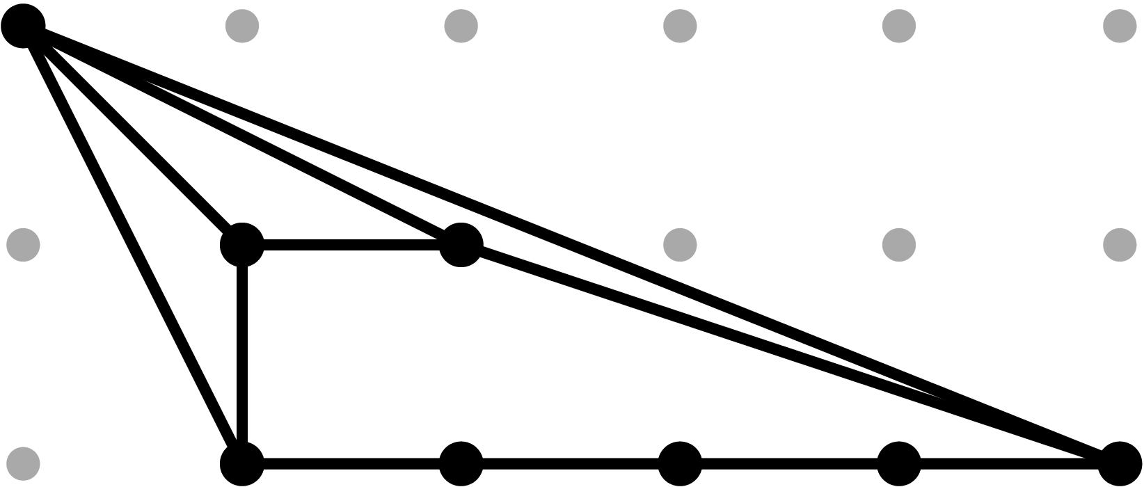
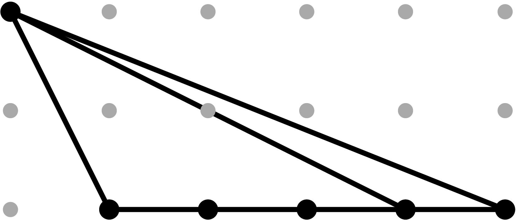
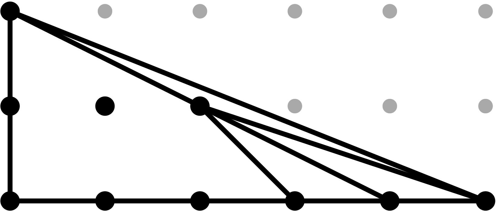
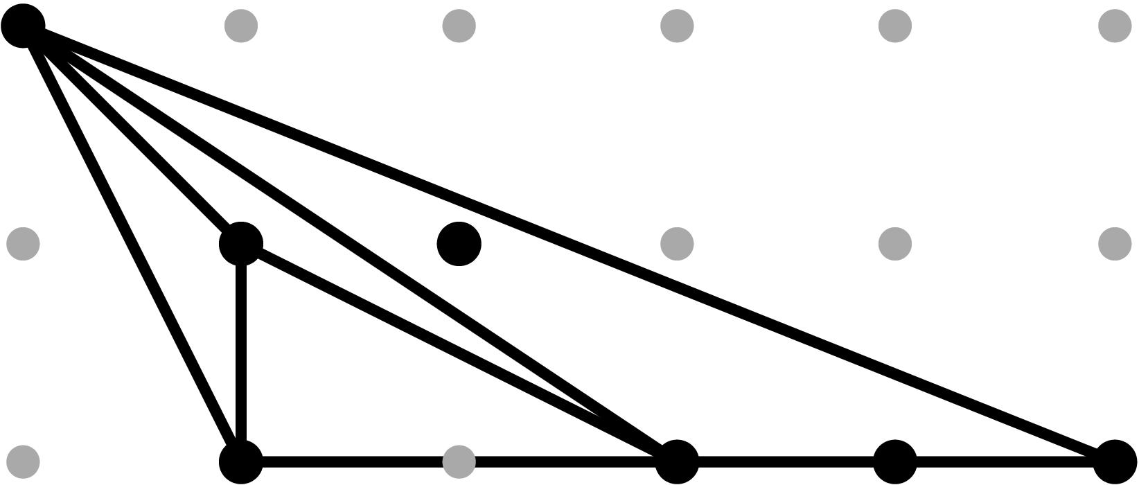
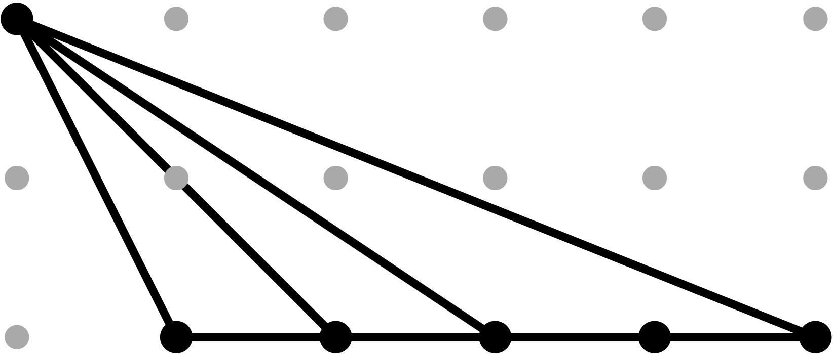
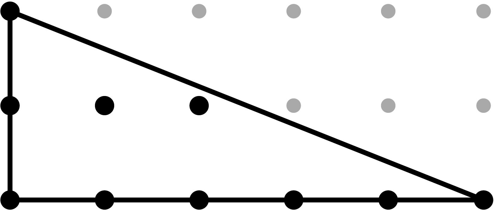
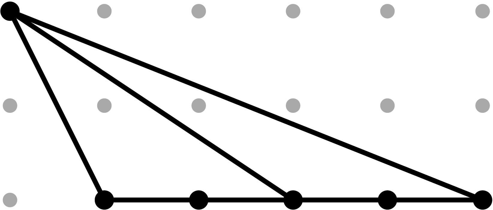
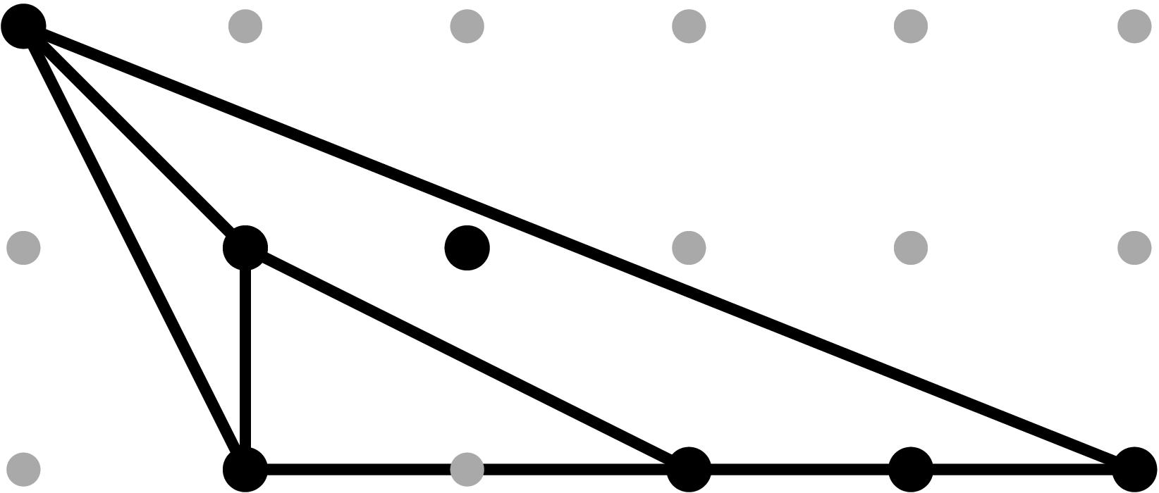
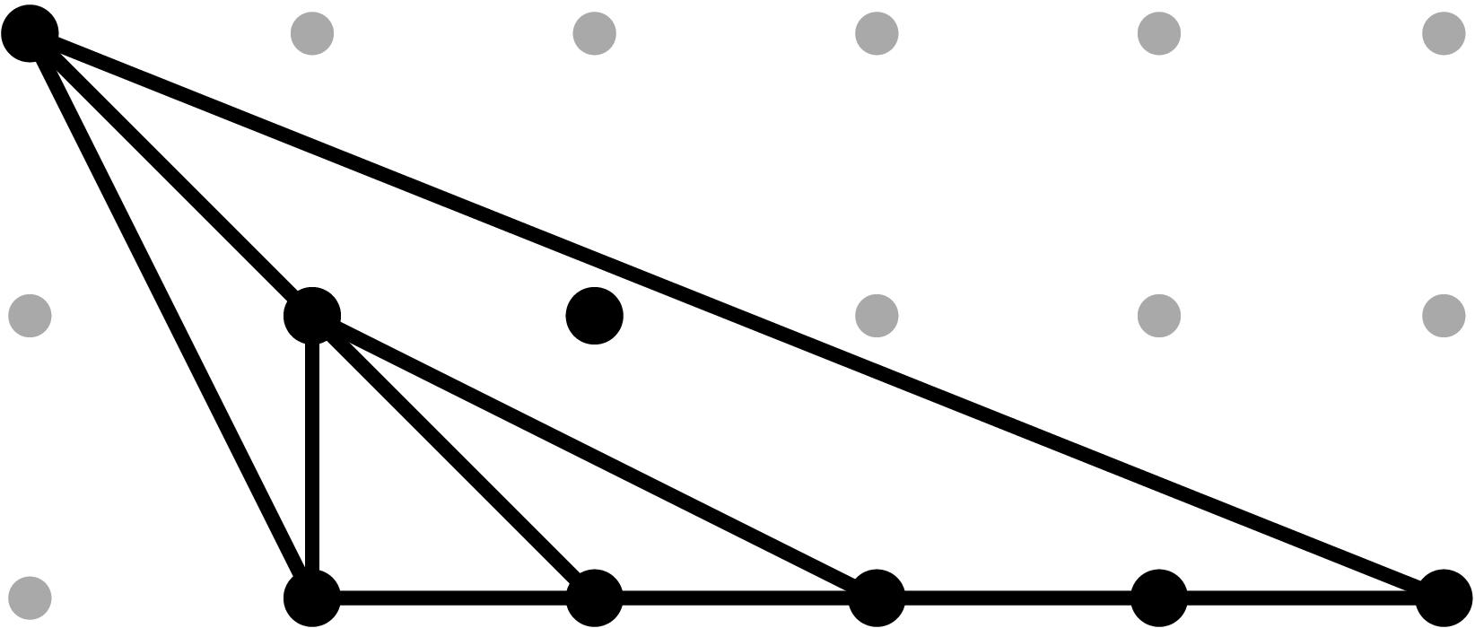
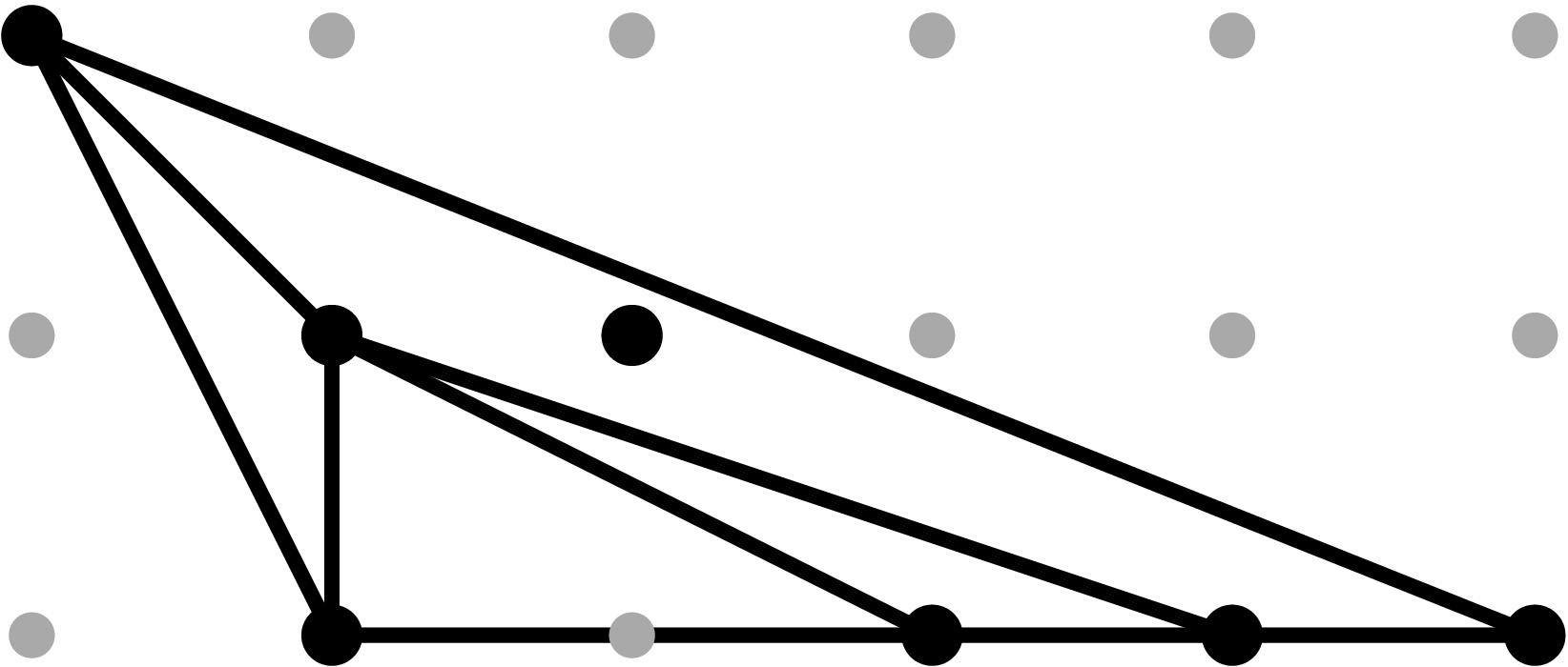
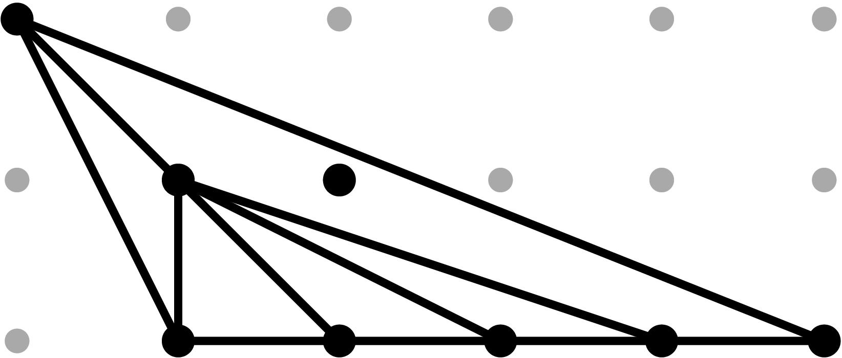
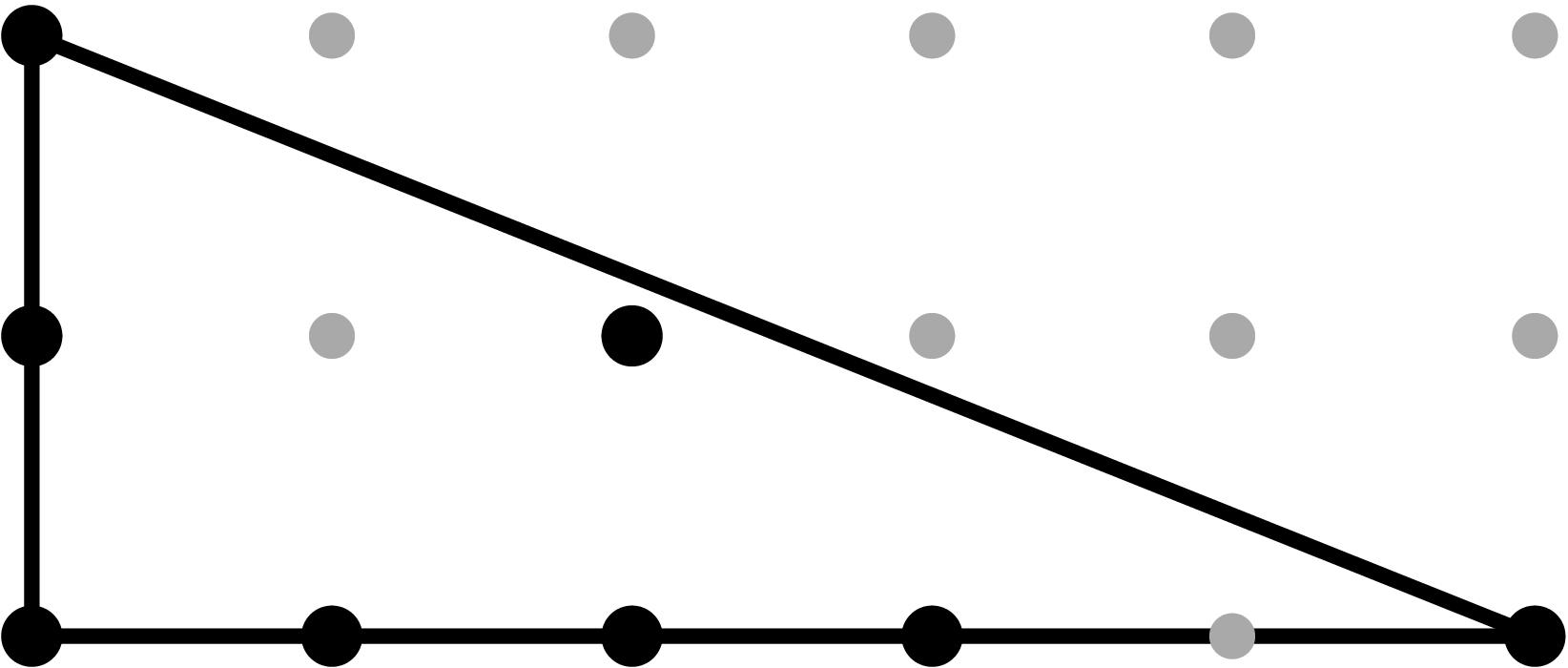
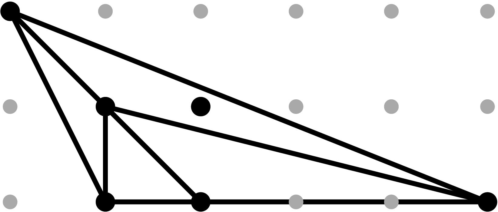
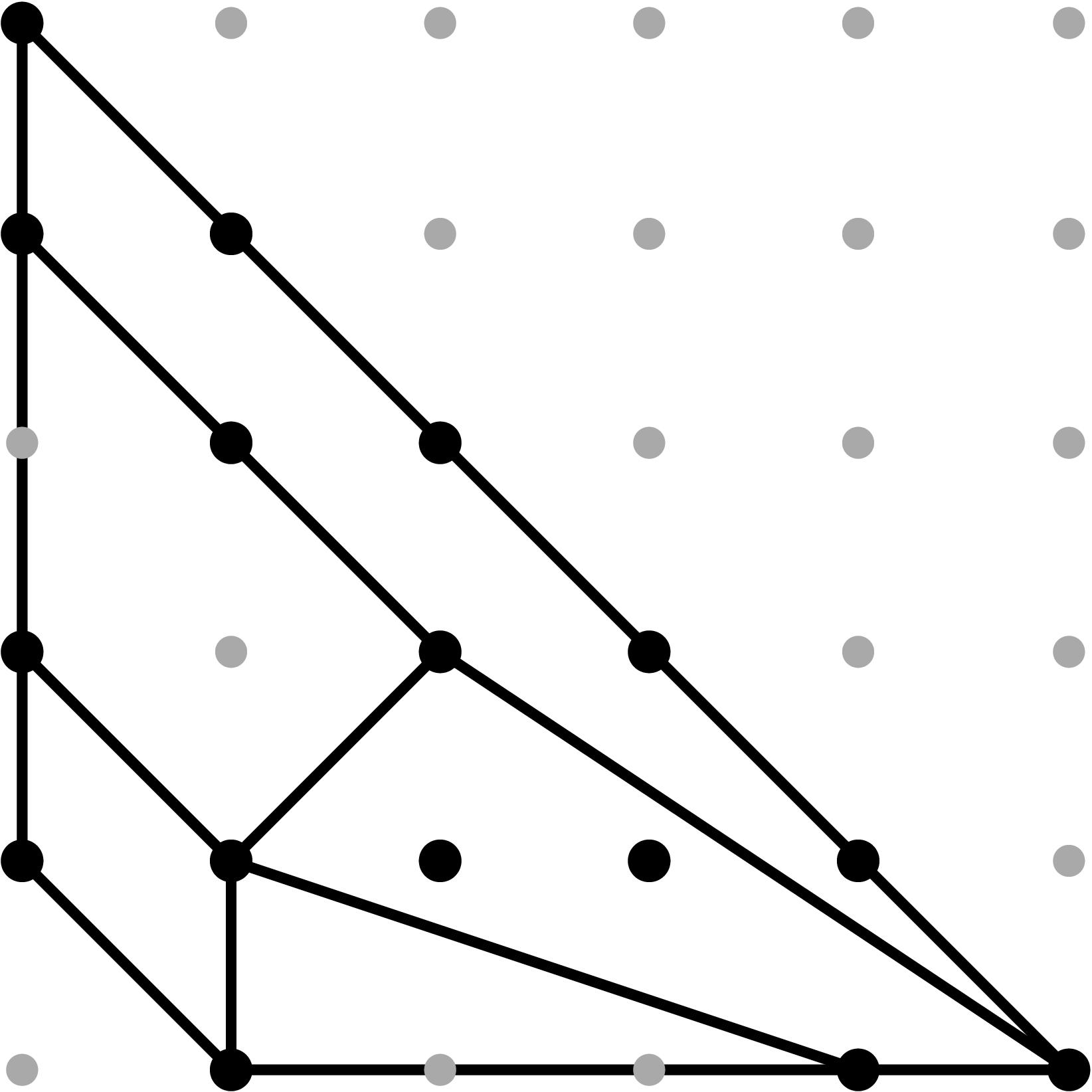
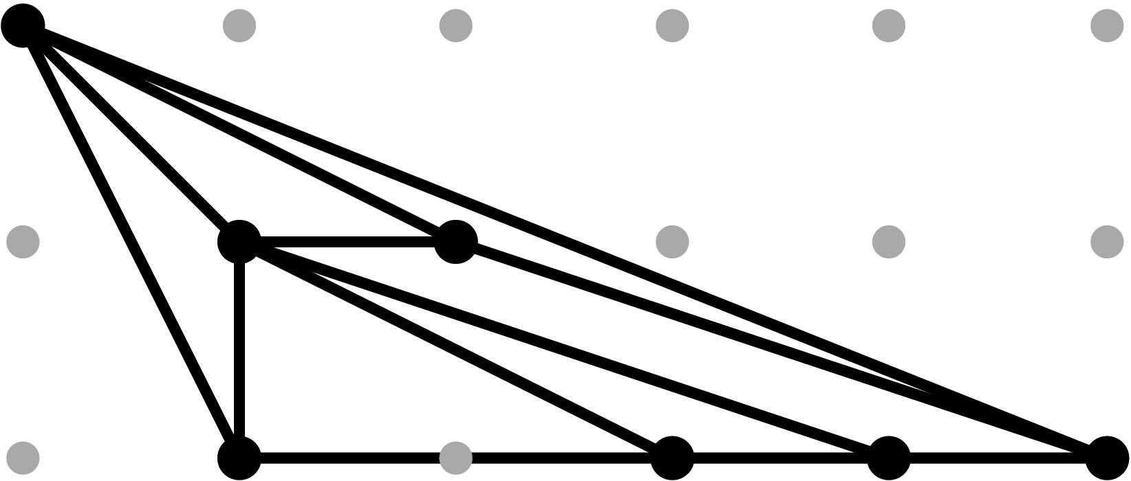
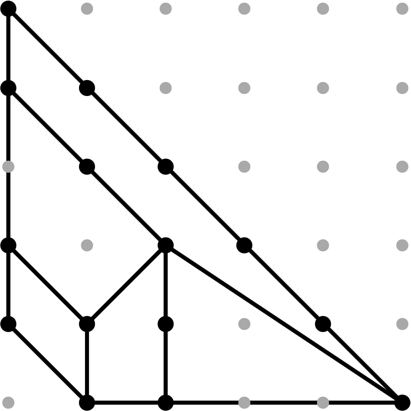
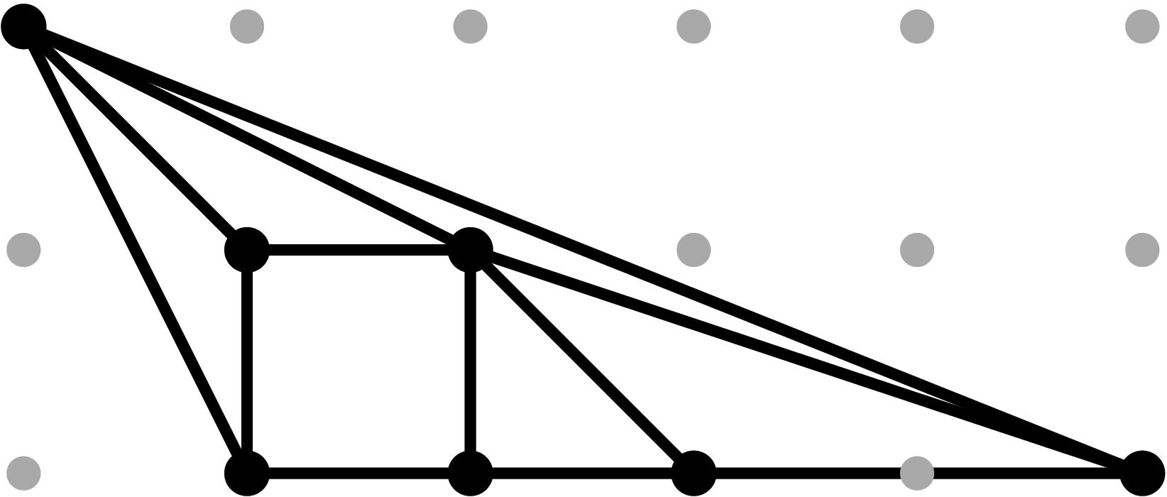
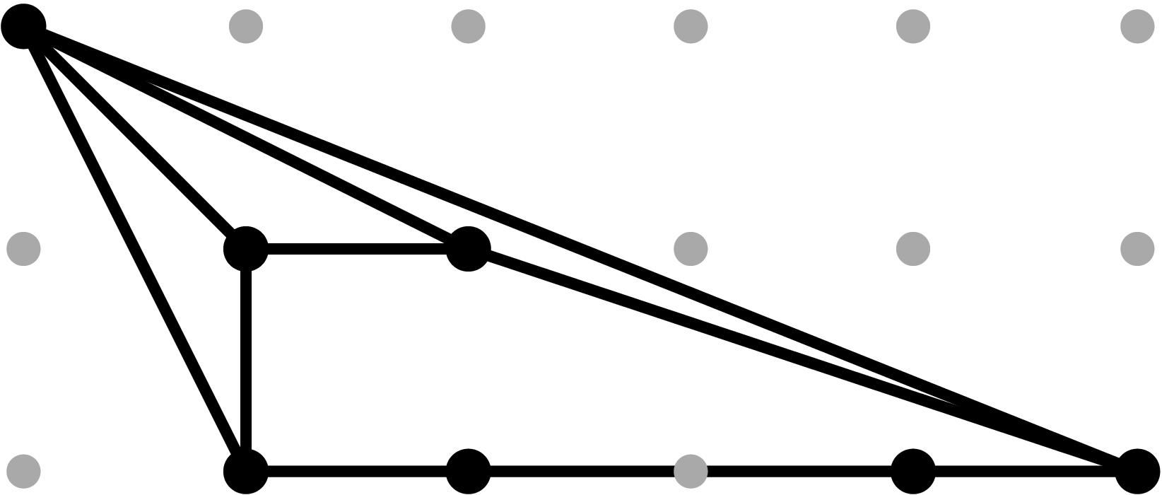
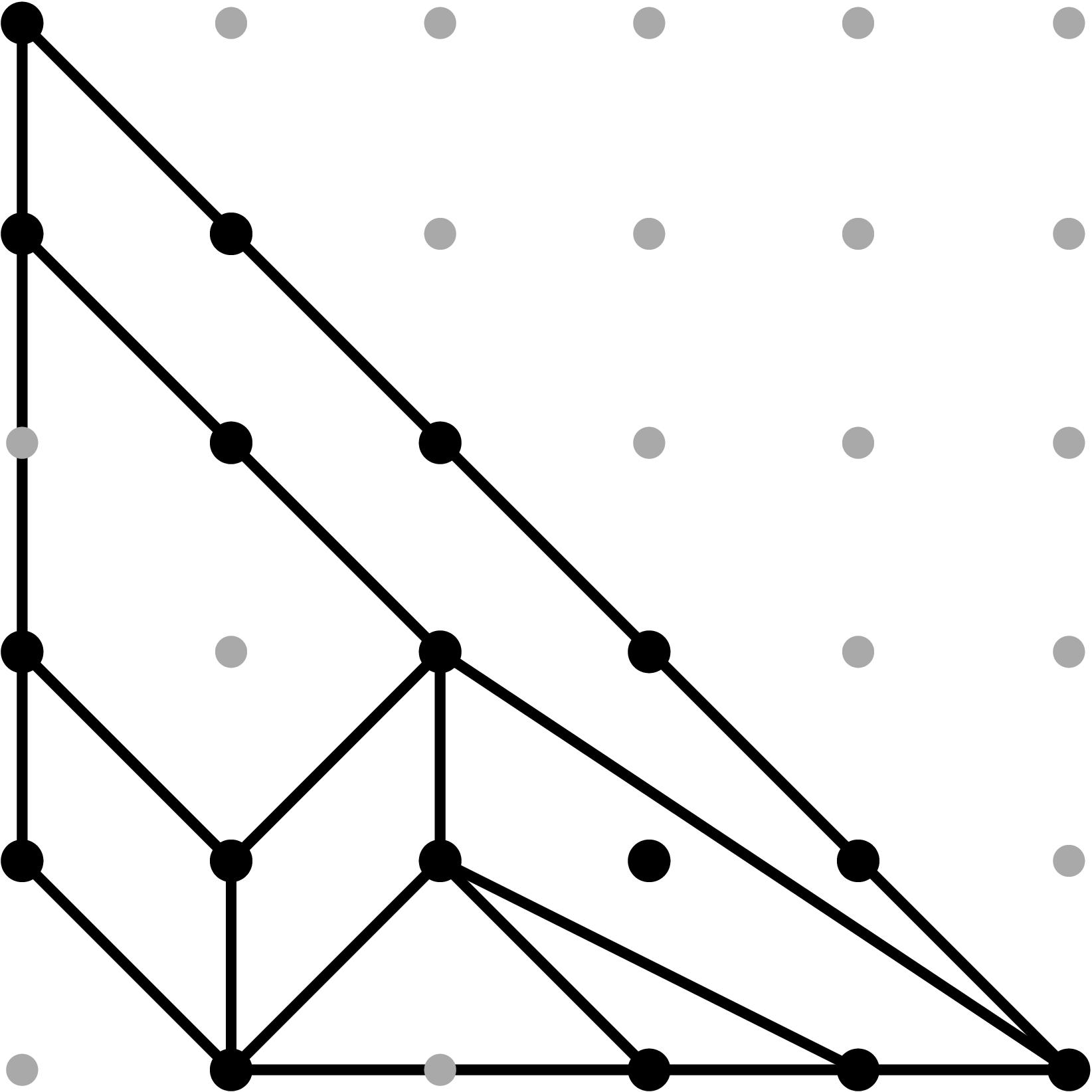
Once the Gröbner fan of the product of all coefficients is computed, we intersect the resulting fan with the Type II Cone, check for possible subdivisions of this cone induced by the fan, and compute the leading terms for each piece in the subdivision. The Type II Cone gets subdivided into 3 and 4 maximal pieces, respectively, as shown in Figure 1. The blue cones have maximal dimension 4, the red cones have dimension 3 and the purple cones have dimension 2. Since we are interested in the relative interior of the Type II Cone, we ignore components of the subdivision lying on the 3 facets.

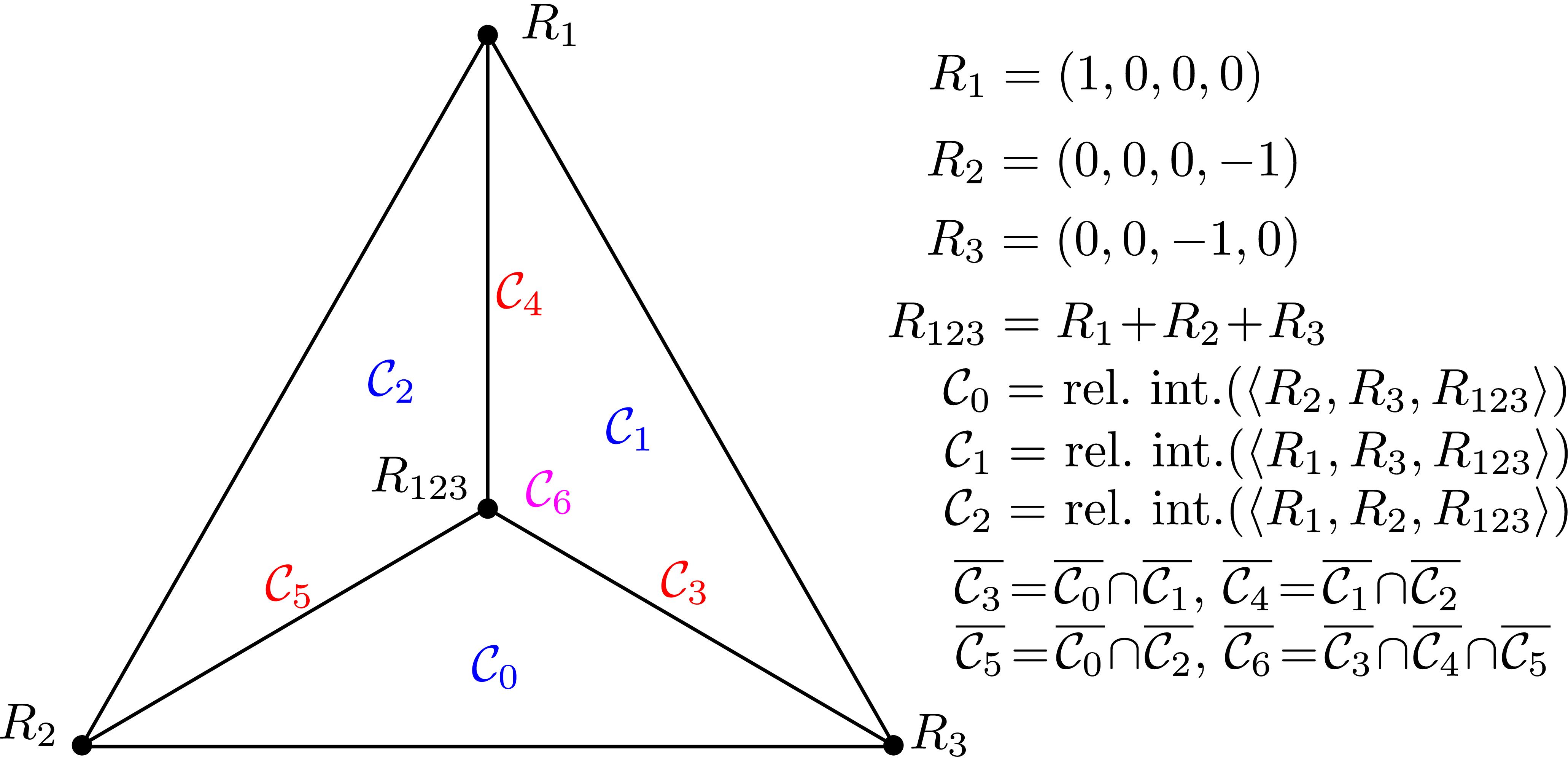
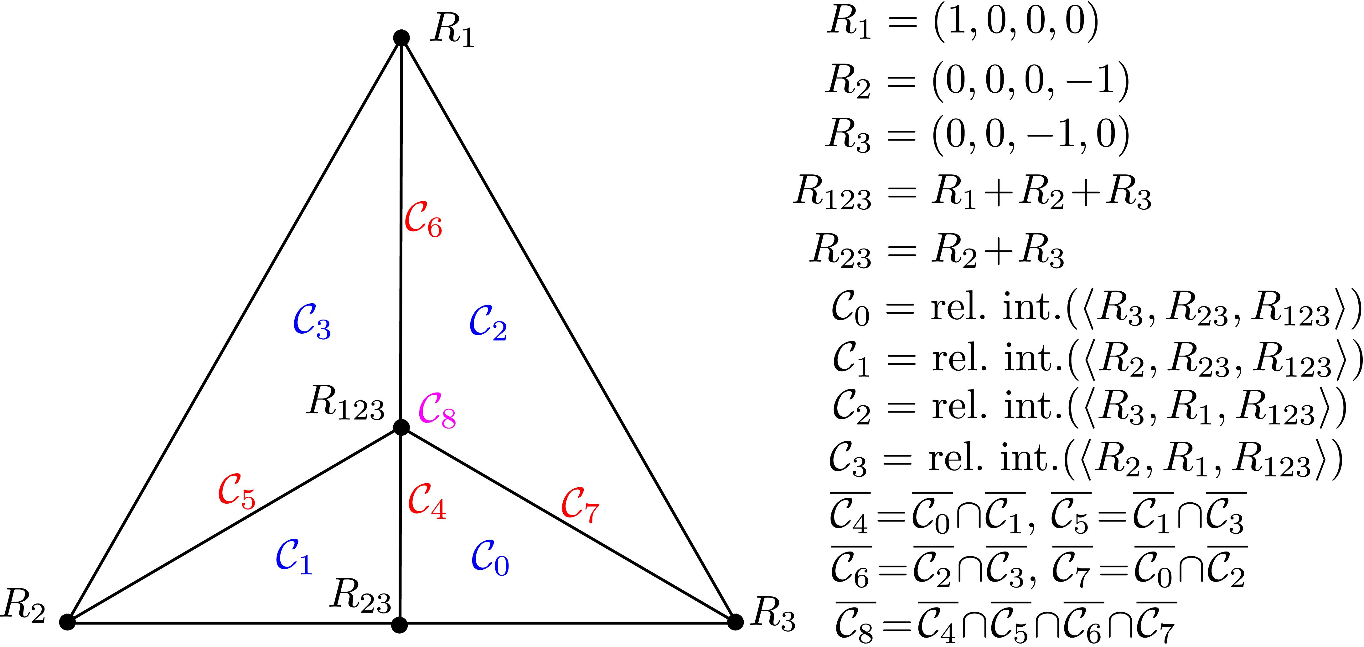Figure 1: From left to right: subdivision of the Type II Cone induced by the Gröbner fans of the coefficients of the (x,z)- and (y,z)-projections, with the coordinates of each extremal ray, after moding out by the all-ones vector.

The following scripts were used to compute the subvisions from Figure 1 and group together the cones yielding the same leading term expressions. In order to determine the leading terms of each of the 17 relevant coefficients, we pick a sample point on each cone. For each cone we always take the sum of its extremal rays, moding out by the all-ones vector to make all entries non-positive and taking the corresponding primitive representative. This will facilitate the construction of examples to determine the possible Newton subdivisions for each projection.

Plain text output of the leading terms of all 3 relevant coefficients of the (y,z)-projection (the indices of the cones correspond to the cones in the subdivision induced by the (y,z) projection, since it is finer than the one induced by the (x,z) projection.)
Sage script that computes the subdivision induced by the 3 relevant coefficients of the (x,z)-projection, the extremal rays and the Leading terms for each of the 7 cones, grouping cones with the same leading terms. Table 1 collects the output data.
Plain text output of the leading terms of all 14 relevant coefficients of the (y,z)-projection.
Sage script that computes the subdivision induced by the 14 relevant coefficients of the (y,z)-projection, the extremal rays and the Leading terms for each of the 9 cones, grouping cones with the same leading terms. Table 2 collects the output data.
Sage script that computes relevant combinatorial data of the common refinement of both subdivisions (f-vector, extremal rays, lineality space and H-representation of all pieces), sample points on each cone and the associated leading terms.
Sage object recording all 8 pieces of the subdivision of the Type II Cone (as polyhedral objects).
Sage object recording the leading terms for all 3 relevant coefficients in the (x,z)-projection for each piece in the subdivision.
Sage object recording the leading terms for all 14 relevant coefficients in the (y,z)-projection for each piece in the subdivision.

Tables 1 and 2 collect the expressions of the leading terms, factored to indicate situations where the expected leading terms have higher valuation than expected. The cone labels agree with those in Figure 1. Caveat: The computations are valid for any characteristic of the residue field, except 2 and 3.

**Table 1: Expected leading terms for each coefficient of the (x,z)-projections and each of the 6 relevant cones in the leftmost subdivision of the Type II Cone in Figure 1.**
Monomials	Leading Terms	Cones
x⁴	(-2) * b4^2	[0, 1, 2, 3, 4, 5, 6]
x³	(-1) * b2^2 * b5^2 (-1) * b34^2 * b5^2 (-1) * b5^2 * (b34^2 + b2^2) b4^4 (-1) * (-b4^2 + b5b2) (b4^2 + b5b2) (-1) (-b4^2 + b5b34) (b4^2 + b5b34) (-1) (-b4^4 + b5^2b34^2 + b5^2b2^2)	[1] [2] [4] [0] [3] [5] [6]
x²	(2) * b2^2 * b4^2 * b5^2	[0, 1, 2, 3, 4, 5, 6]

**Table 2: Expected leading terms for each coefficient of the (y,z)-projections and each of the nine relevant cones in the rightmost subdivision of the Type II Cone in Figure 1.**
Monomials	Leading Terms	Cones
y ⁴	(2) * b2^2 * b5^3 (2) * b34^2 * b5^3 (2) * b5^3 * (b34^2 + b2^2)	[0, 2, 7] [1, 3, 5] [4, 6, 8]
y³ z	(-2) * b4^2 * b5^3	[0, 1, 2, 3, 4, 5, 6, 7, 8]
y² z²	(4) * b5^5	[0, 1, 2, 3, 4, 5, 6, 7, 8]
y z³	(-4) * b5^5	[0, 1, 2, 3, 4, 5, 6, 7, 8]
z⁴	b5^5	[0, 1, 2, 3, 4, 5, 6, 7, 8]
y³	b2^4 * b5^6 (-1) * b2^2 * b4^4 * b5^4 b2^2 * b5^4 * (-b4^2 + b5b2) (b4^2 + b5b2) b34^4 b5^6 b5^6 * (b34^2 + b2^2)^2 (-1) * b34^2 * b4^4 * b5^4 (-1) * b4^4 * b5^4 * (b34^2 + b2^2) b34^2 * b5^4 * (-b4^2 + b5b34) (b4^2 + b5b34) b5^4 (b34^2 + b2^2) * (-b4^4 + b5^2b34^2 + b5^2b2^2)	[2] [0] [7] [3] [6] [1] [4] [5] [8]
y² z	(2) * b2^2 * b4^2 * b5^6 (-6) * b34^2 * b4^2 * b5^6 (-2) * b4^2 * b5^6 * (3*b34^2 - b2^2)	[0, 2, 7] [1, 3, 5] [4, 6, 8]
y z²	(-3) * b2^2 * b4^2 * b5^6 (9) * b34^2 * b4^2 * b5^6 (3) * b4^2 * b5^6 * (3*b34^2 - b2^2)	[0, 2, 7] [1, 3, 5] [4, 6, 8]
z³	b2^2 * b4^2 * b5^6 (-3) * b34^2 * b4^2 * b5^6 (-1) * b4^2 * b5^6 * (3*b34^2 - b2^2)	[0, 2, 7] [1, 3, 5] [4, 6, 8]
y²	(-4) * b2^2 * b34^2 * b4^4 * b5^7	[0, 1, 2, 3, 4, 5, 6, 7, 8]
y z	(2) * b34^2 * b4^6 * b5^7	[0, 1, 2, 3, 4, 5, 6, 7, 8]
z²	(-1) * b34^2 * b4^6 * b5^7	[0, 1, 2, 3, 4, 5, 6, 7, 8]
y	b2^2 * b34^2 * b4^8 * b5^8	[0, 1, 2, 3, 4, 5, 6, 7, 8]
z	(-1) * b2^2 * b34^2 * b4^8 * b5^8	[0, 1, 2, 3, 4, 5, 6, 7, 8]

The previous scripts allow us to predict the expected height of each lattice point in the truncated Newton polytopes of the (x,z)- and (y,z)-projection (involving only the 17 relevant monomials, hence to determine the Newton subdivisions.) However, the combinatorial types of the (y,z)-Newton subdivision will vary within a given cone. The following scripts allow us to compute the corresponding Gröbner fans.

Sage script to compute all Gröbner fans for all 8 cones in the Subdivision of the Type II Cone by leading terms of coefficients in the (y,z)-projection.
Sage object: Dictionary of 8 polynomials where we replace each of the 14 coefficient of the truncated (y,z)-equation by its expected leading terms. We will use this to compute the Gröbner fan of the truncated (y,z)-equation.
Sage object: dictionary of all 8 Gröbner fans (one per cone in the right of Figure 1.) Each entry is a polyhedral data-type object in Sage.
Sage object: Dictionary of all Gröbner fans of all 8 polynomials in the previous item. Each fan is given as a dictionary of its maximal cones. Their f-vectors are:
C₀: [1, 10, 34, 52, 38, 12],
C₁: [1, 14, 46, 64, 42, 12],
C₂: [1, 13, 45, 65, 43, 12],
C₃: [1, 19, 59, 74, 43, 11],
C₄: [1, 15, 55, 84, 58, 16],
C₅: [1, 19, 61, 79, 47, 12],
C₆: [1, 19, 66, 91, 56, 14],
C₇: [1, 14, 47, 67, 45, 13],
C₈: [1, 19, 68, 98, 63, 16].

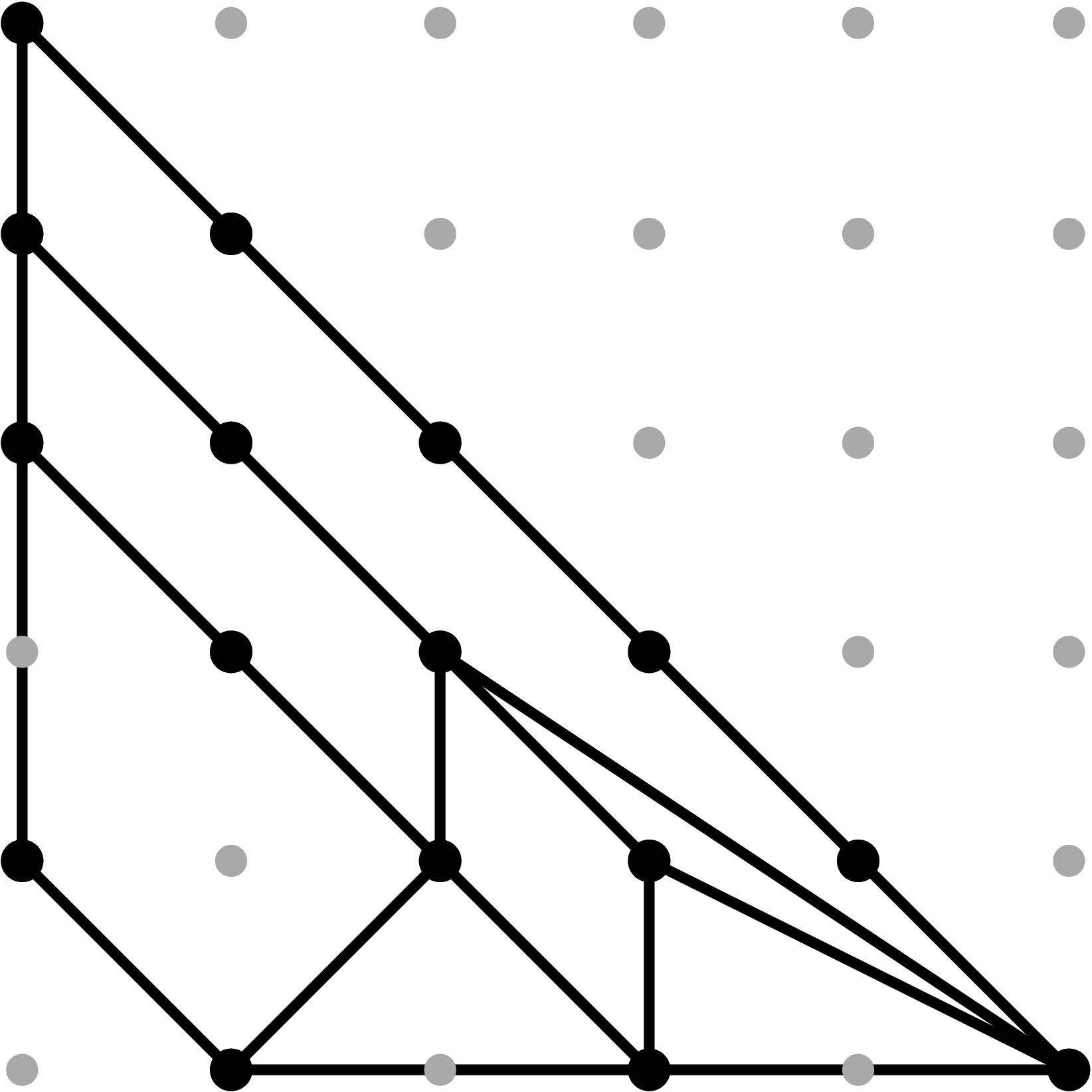
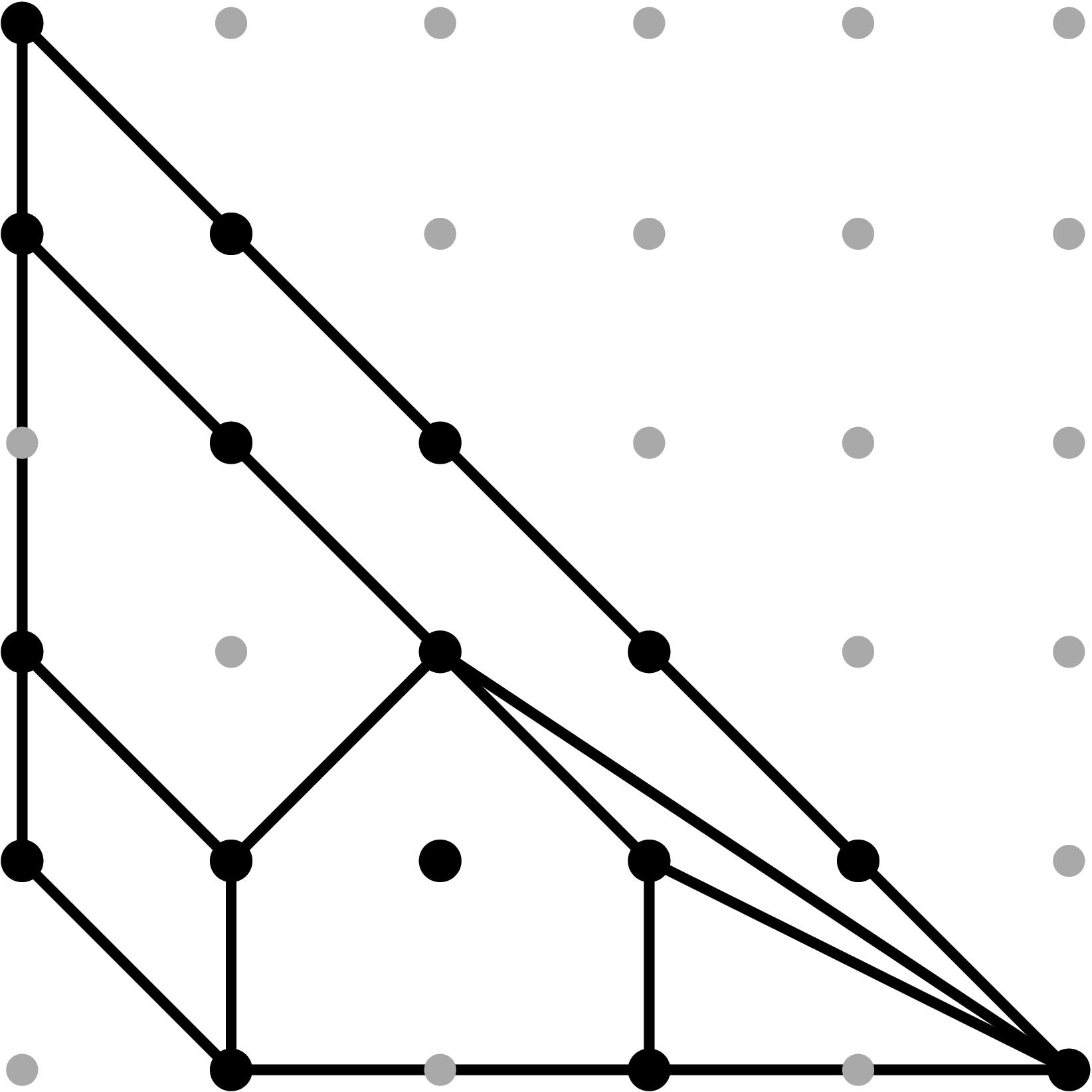
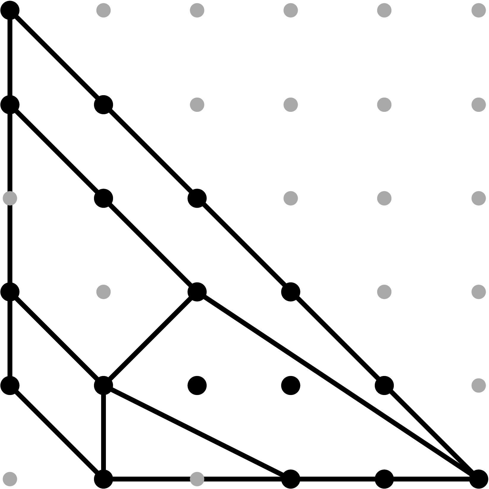
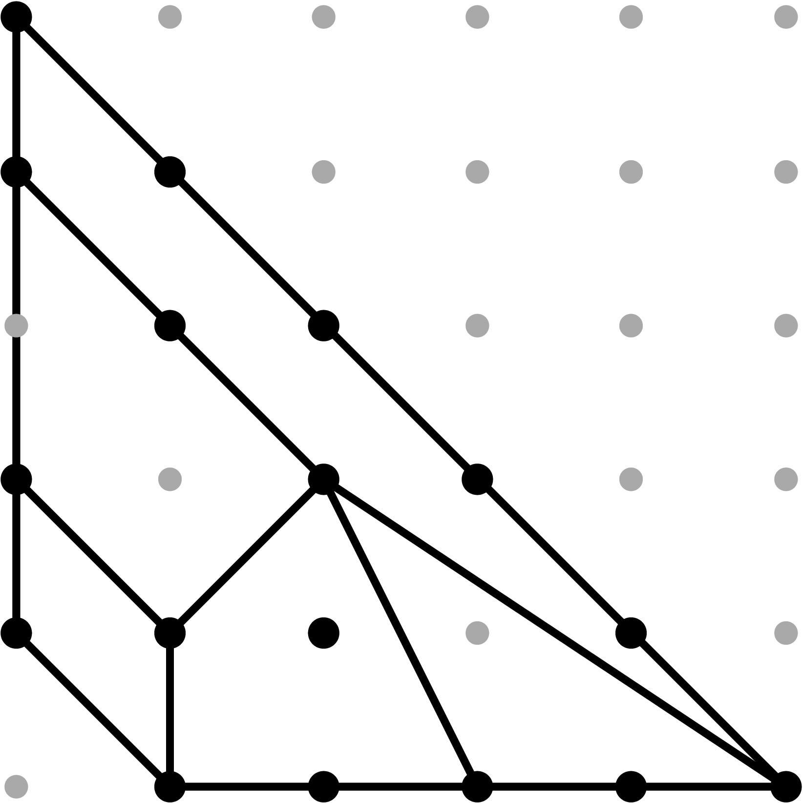
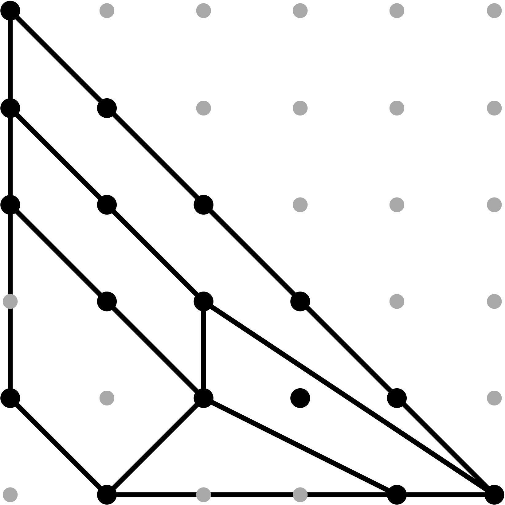
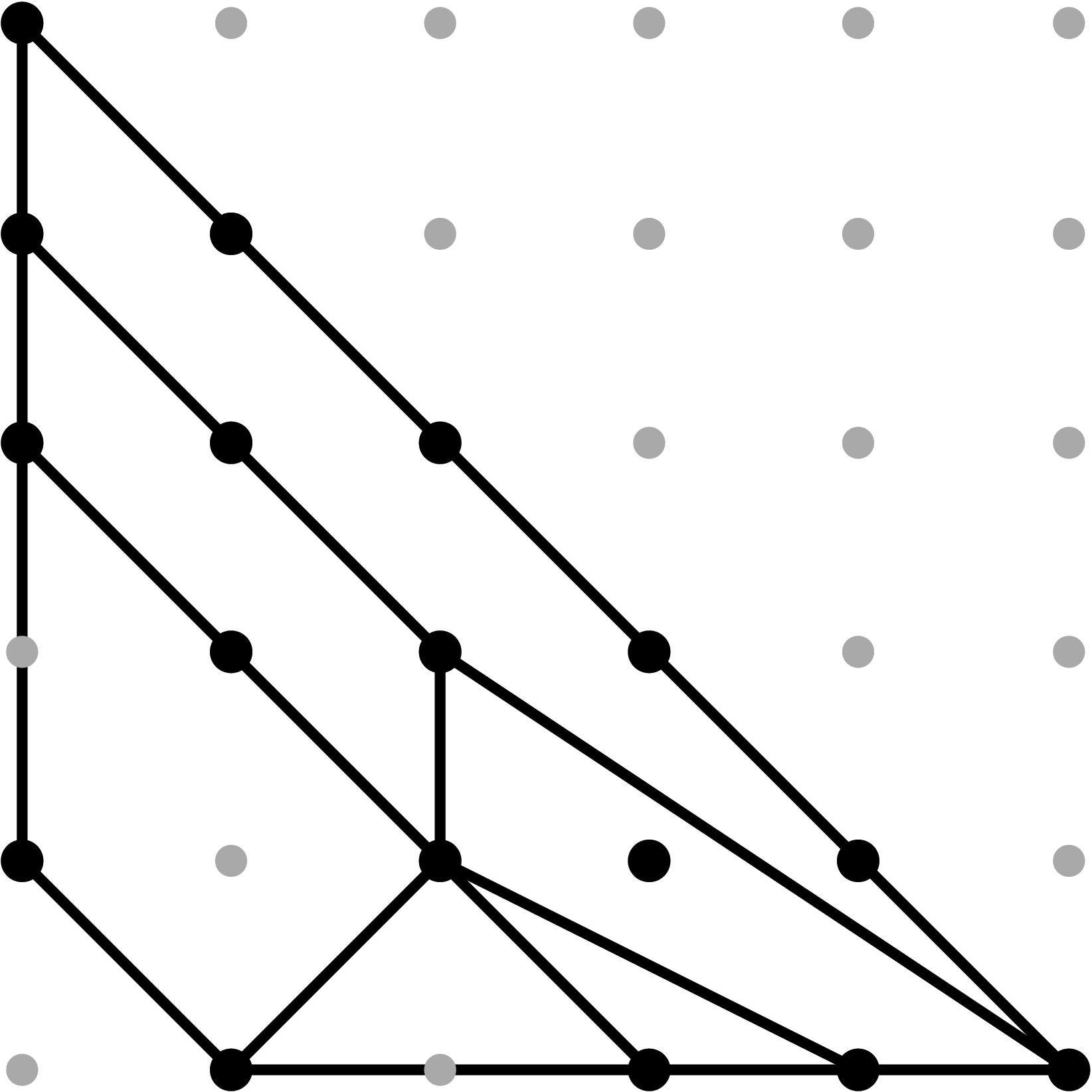
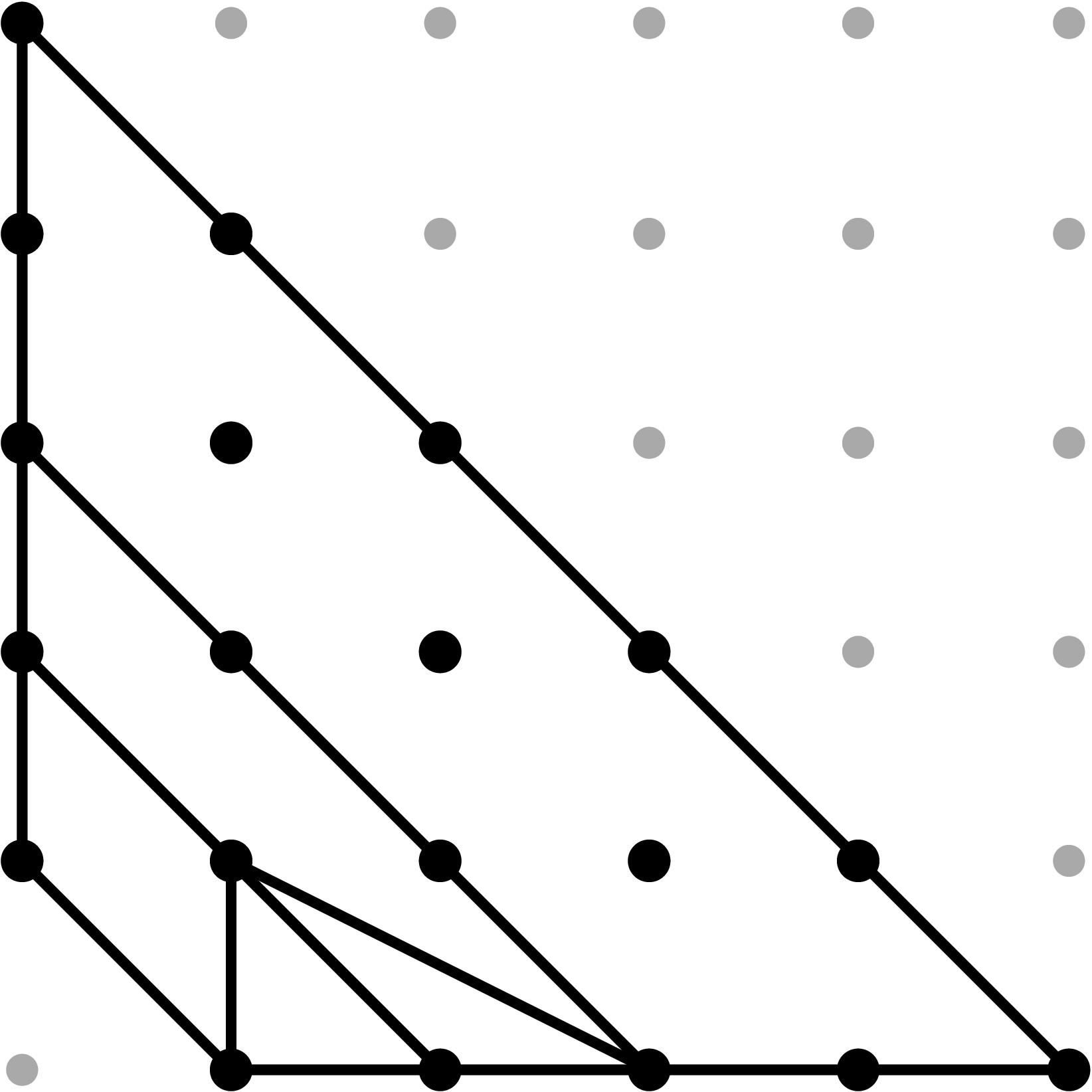
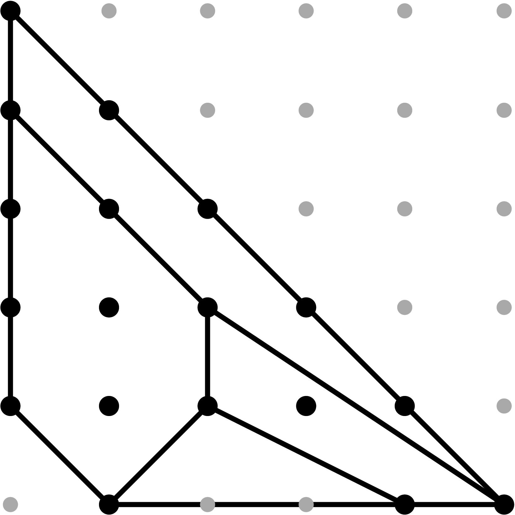
In order to determine the domains of lineality of each combinatorial type, we further subdivide each piece C₀,…, C₈ by the projection of the Gröbner fan in R⁶ of the (y,z)-equation equation in the variables [b₅, b₄, b₃₄, b₂, y, z], to the first 4 parameters. Figure 2 shows the induced refined subdivision: only 2 of the 4 maximal pieces get subdivided. The following scripts compute the subdivisions for each cell, the H-representation, and sample points for each piece, to determine the Newton subdivision by explicit computations on examples, assuming no cancellations on the expected leading terms.

Sage script to compute the refined subdivision of the cone C₀ from Figure 1. The result is a subdivision into 5 cones C_0,0,…, C_0,4 (3 of maximal dimension) as seen in Figure 2.
Sage script to compute the refined subdivision of the cone C₁ from Figure 1. The result is the trivial subdivision, as seen in Figure 2.
Sage script to compute the refined subdivision of the cone C₂ from Figure 1. The result is a subdivision into 3 cones C_2,0,…, C_2,2 (2 of maximal dimension) as seen in Figure 2.
Sage script to compute the refined subdivision of the cone C₃ from Figure 1. The result is the trivial subdivision, as seen in Figure 2.
Sage script to compute the refined subdivision of the cone C₄ from Figure 1. The result is the trivial subdivision, as seen in Figure 2.
Sage script to compute the refined subdivision of the cone C₅ from Figure 1. The result is the trivial subdivision, as seen in Figure 2.
Sage script to compute the refined subdivision of the cone C₆ from Figure 1. The result is the trivial subdivision, as seen in Figure 2.
Sage script to compute the refined subdivision of the cone C₇ from Figure 1. The result is a subdivision into 3 cones C_7,0,…, C_7,2 (2 of maximal dimension) as seen in Figure 2.
Sage script to compute the refined subdivision of the cone C₈ from Figure 1. The result is the trivial subdivision, as seen in Figure 2.

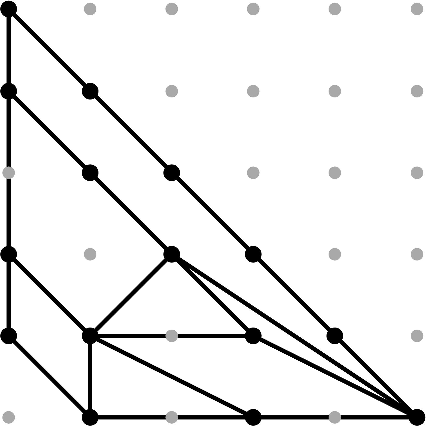
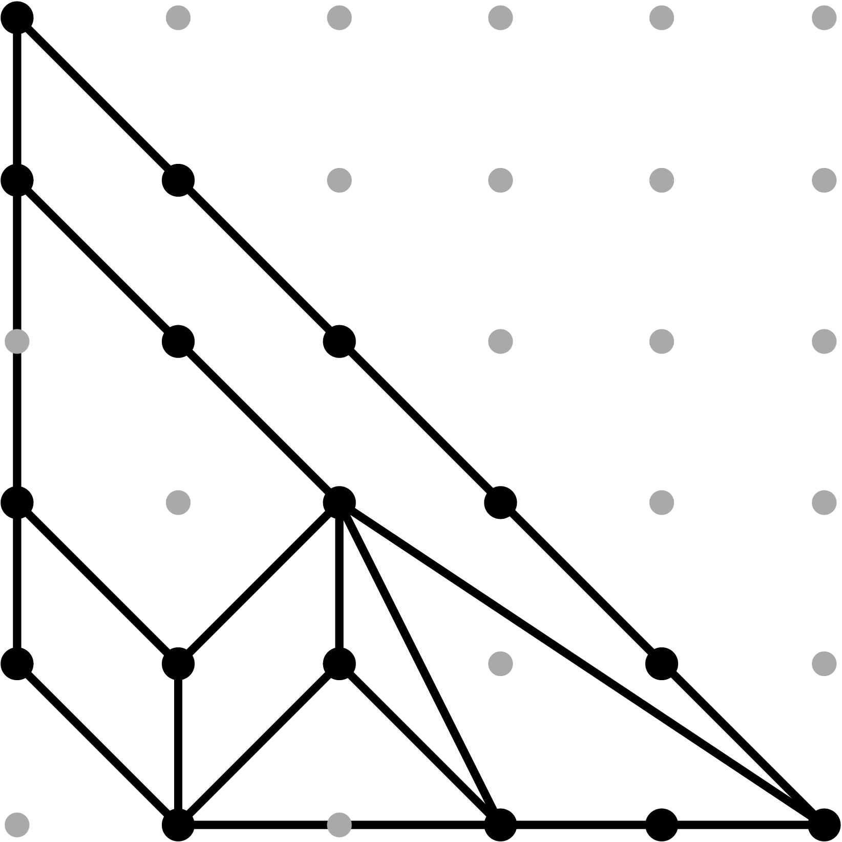
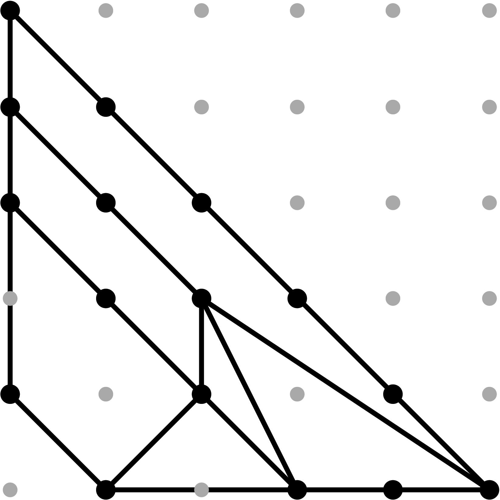
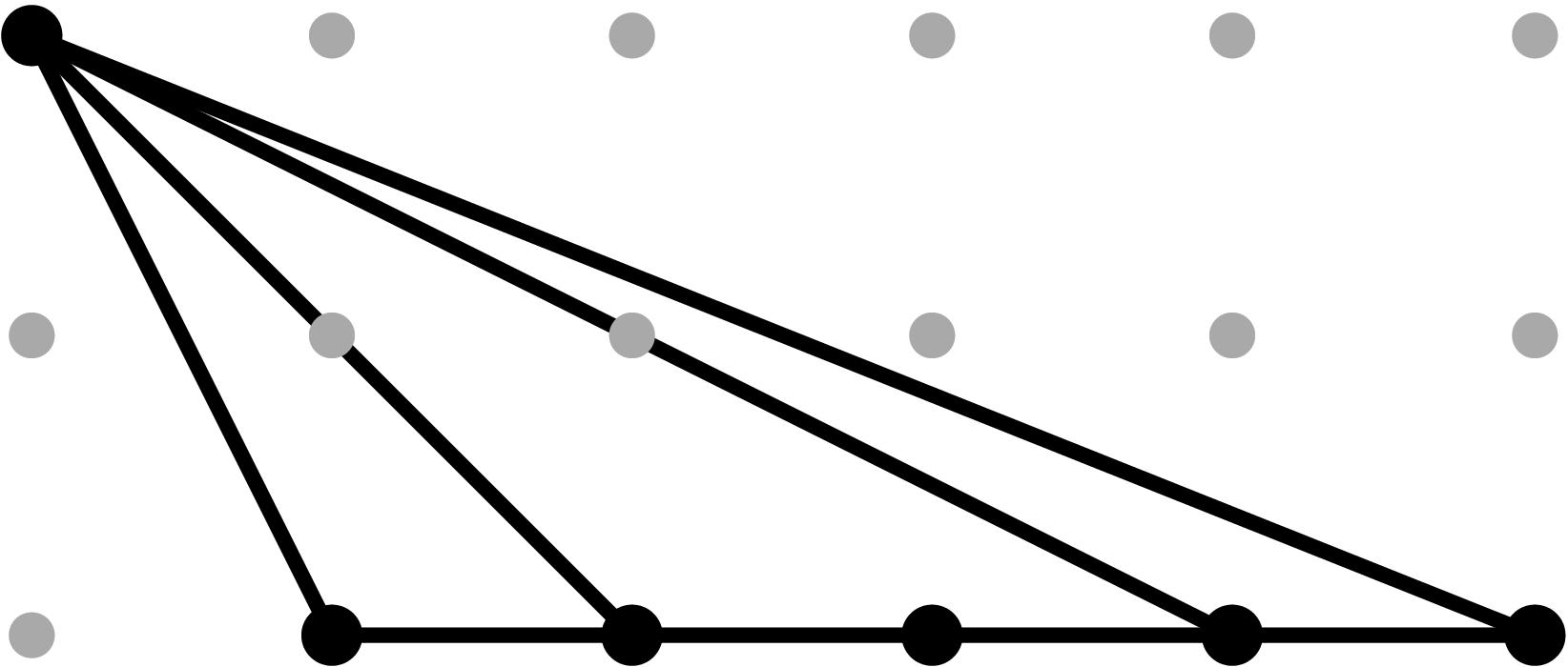
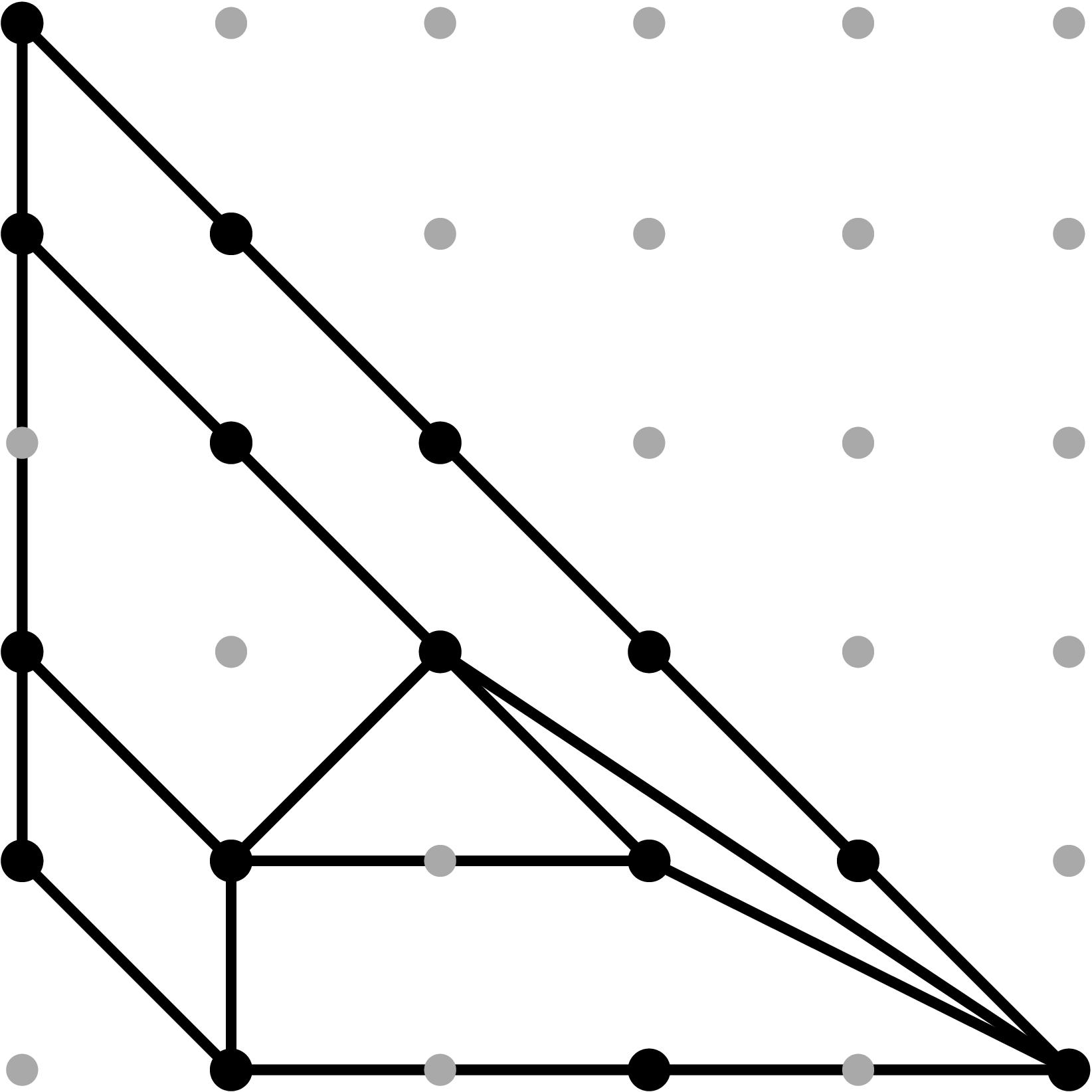
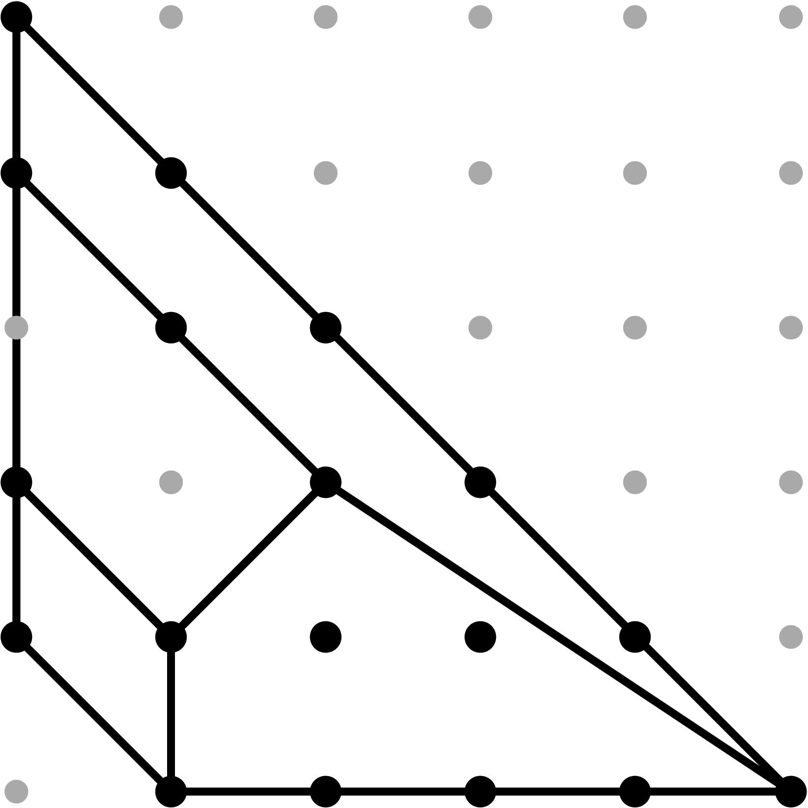
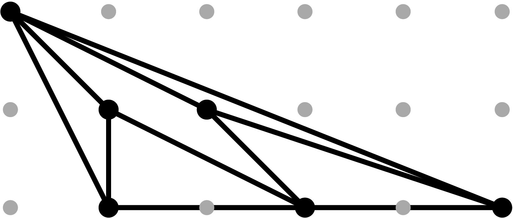
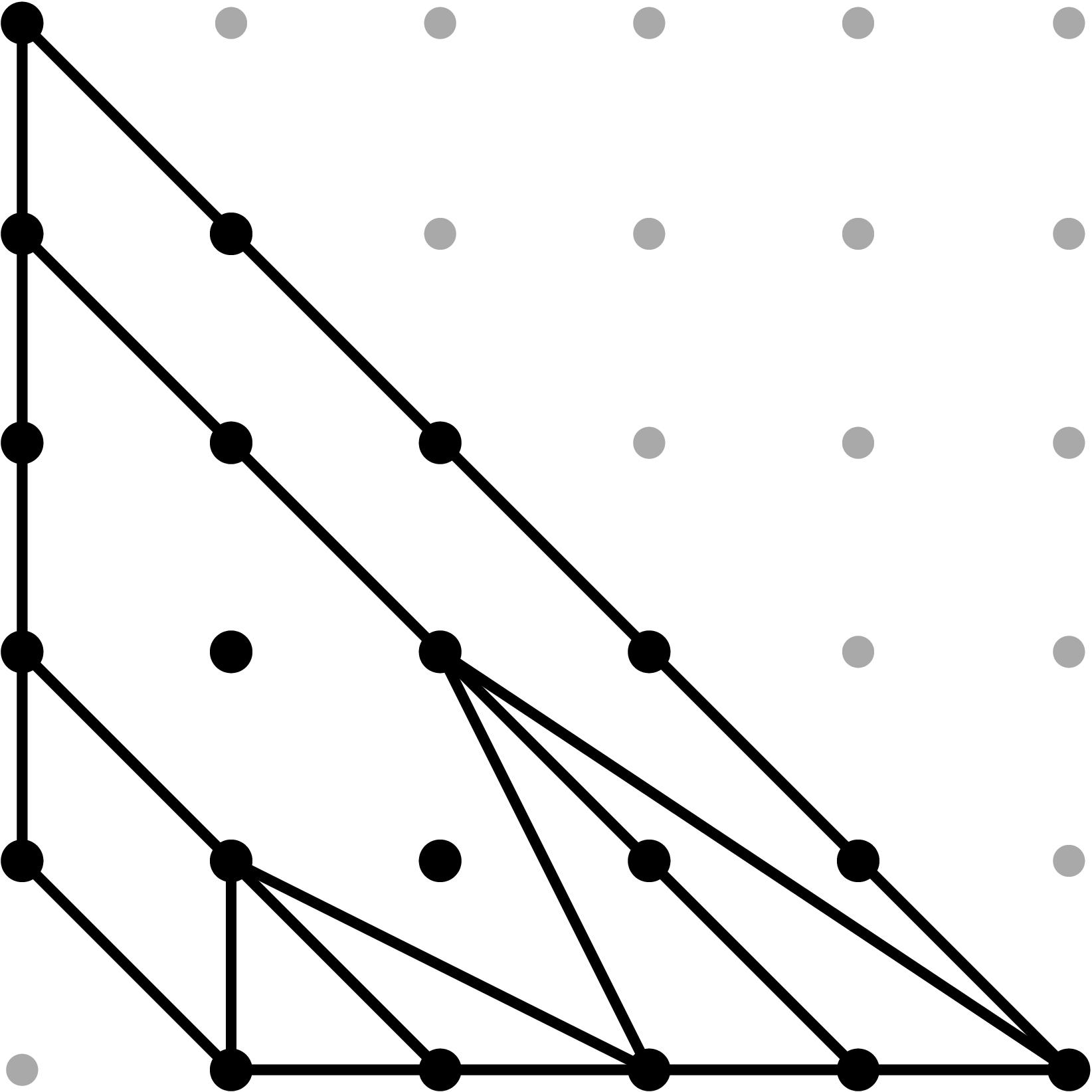
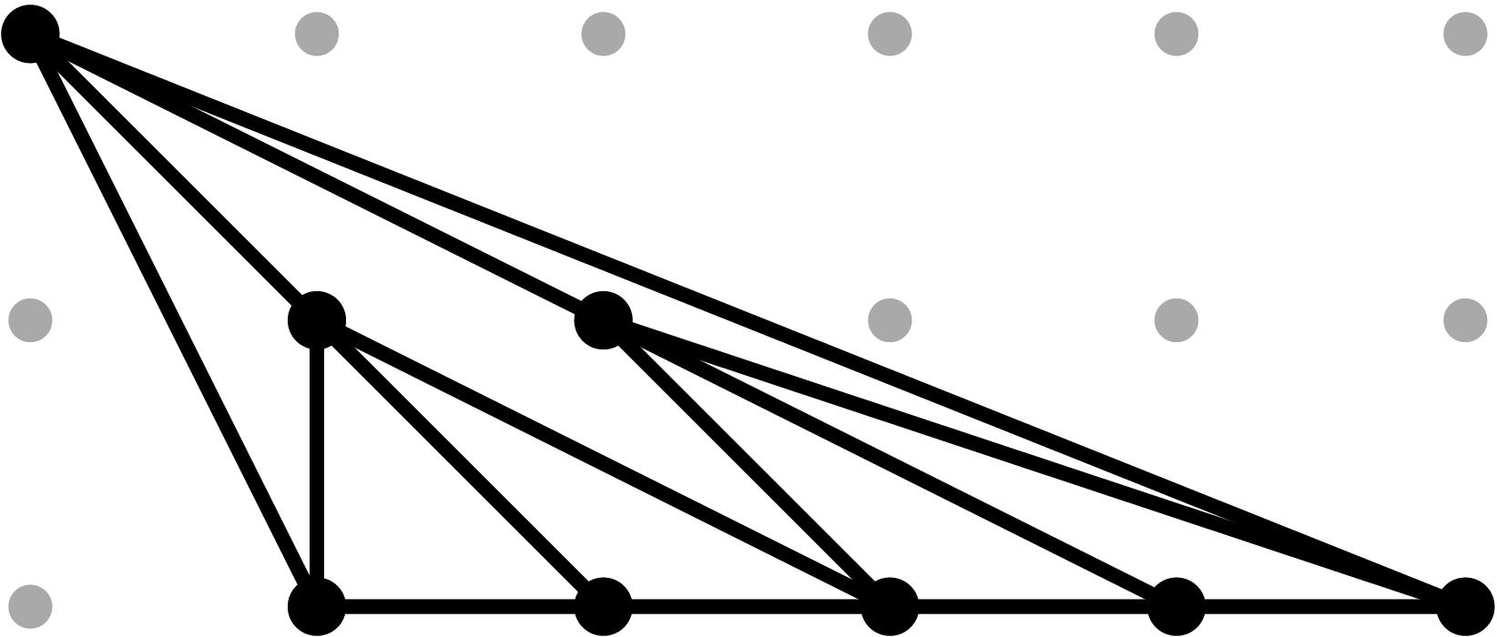
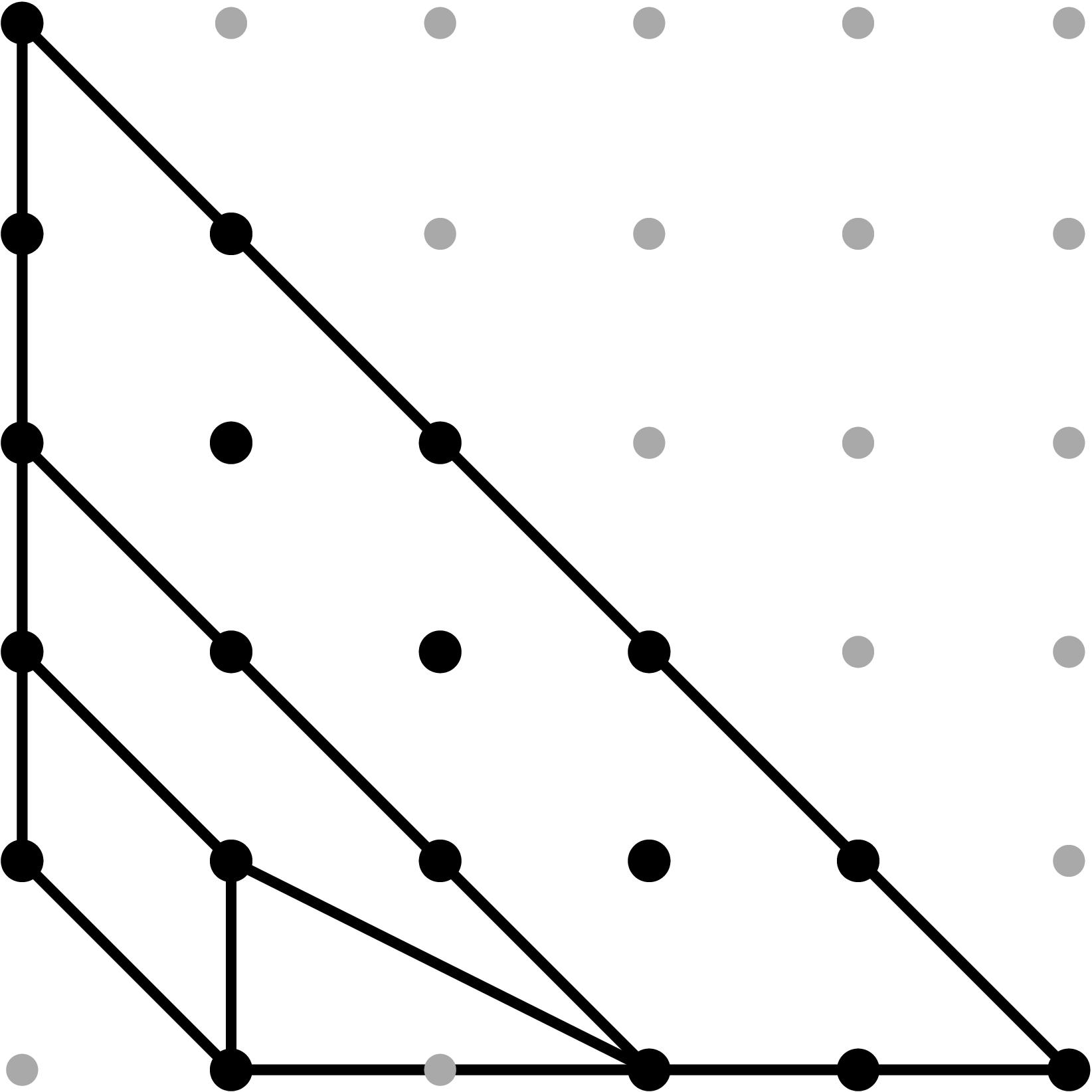
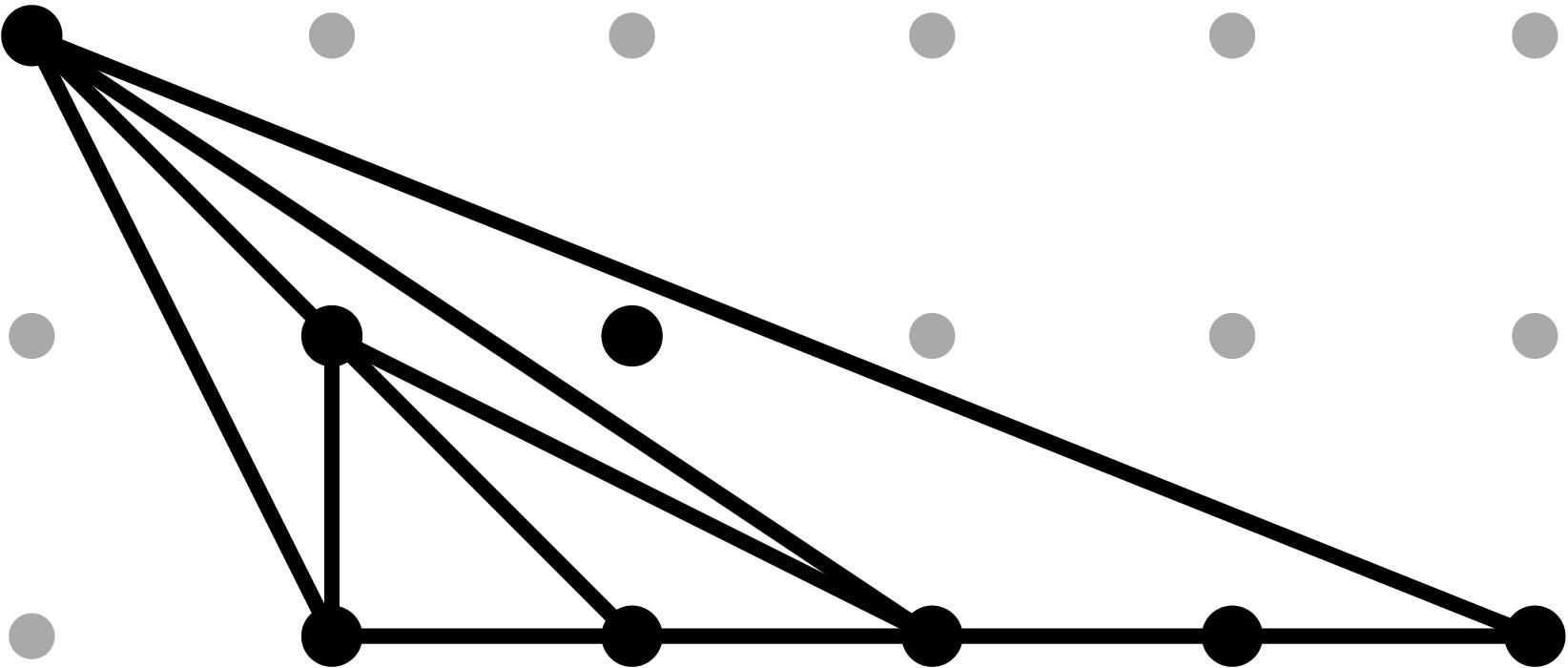
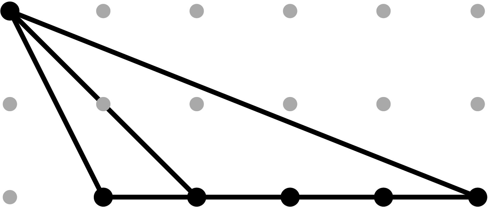
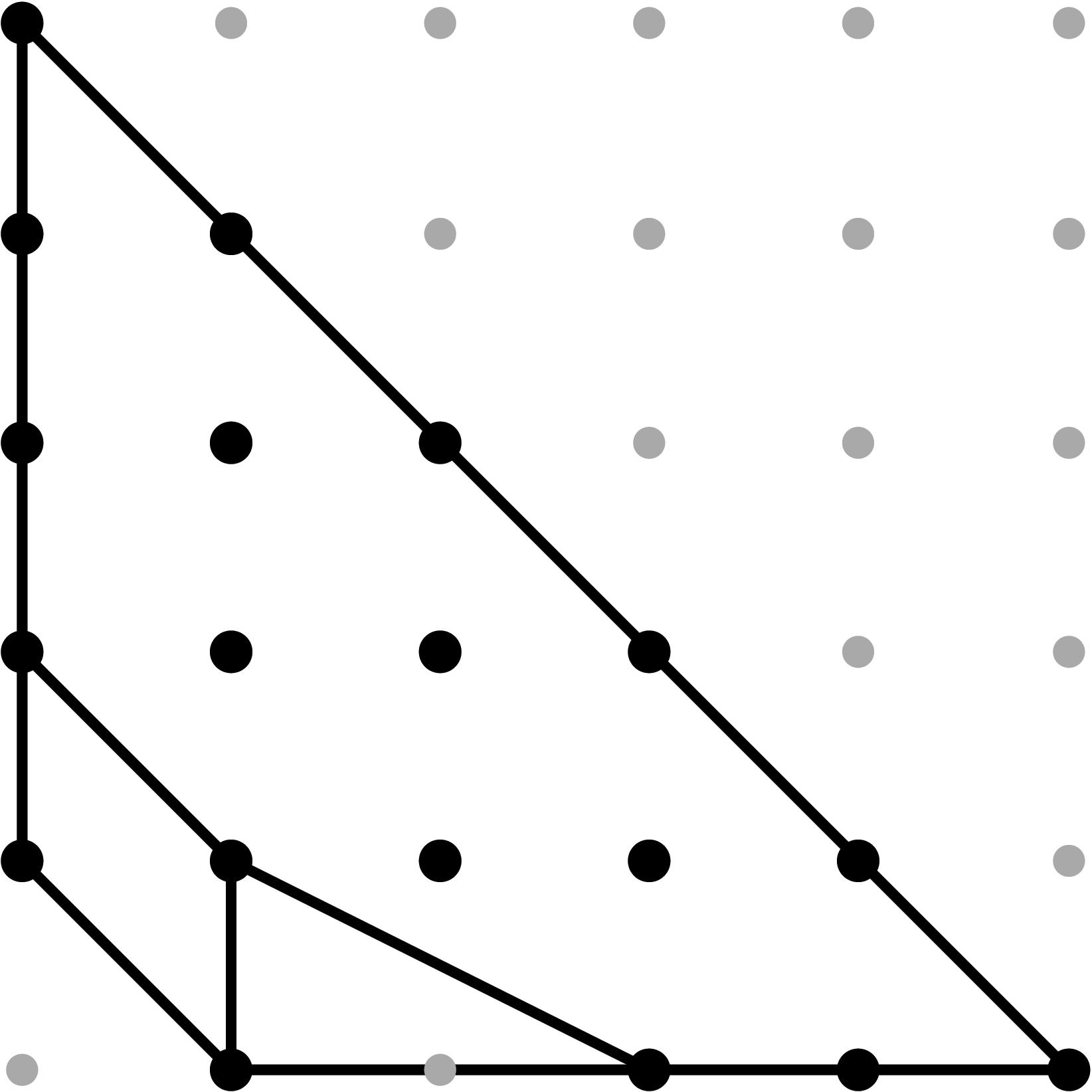
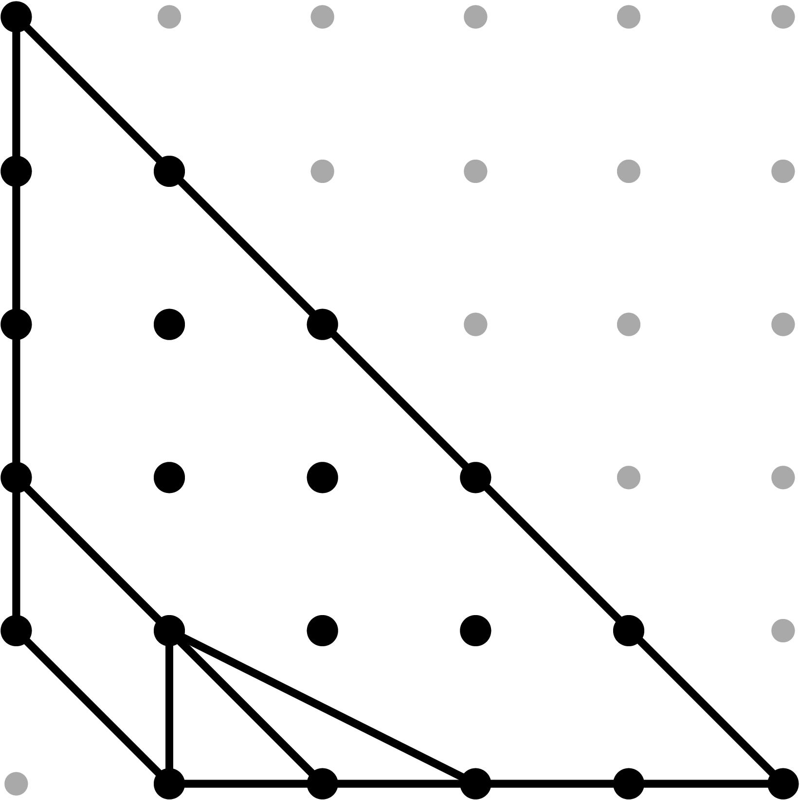
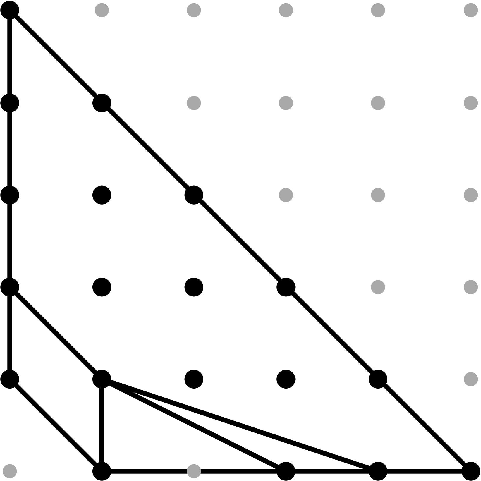
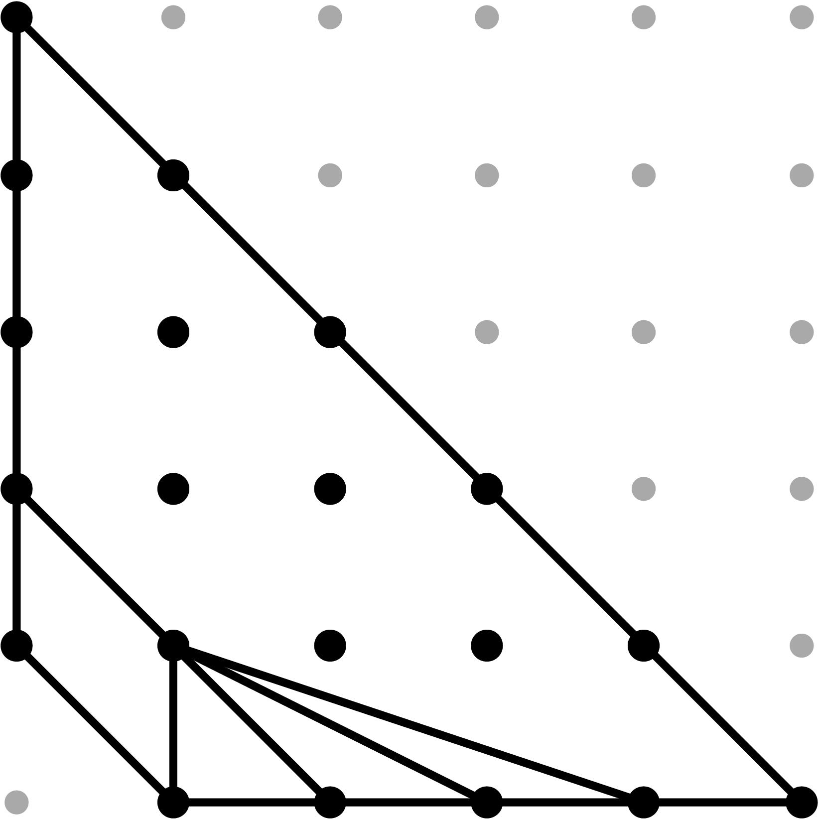
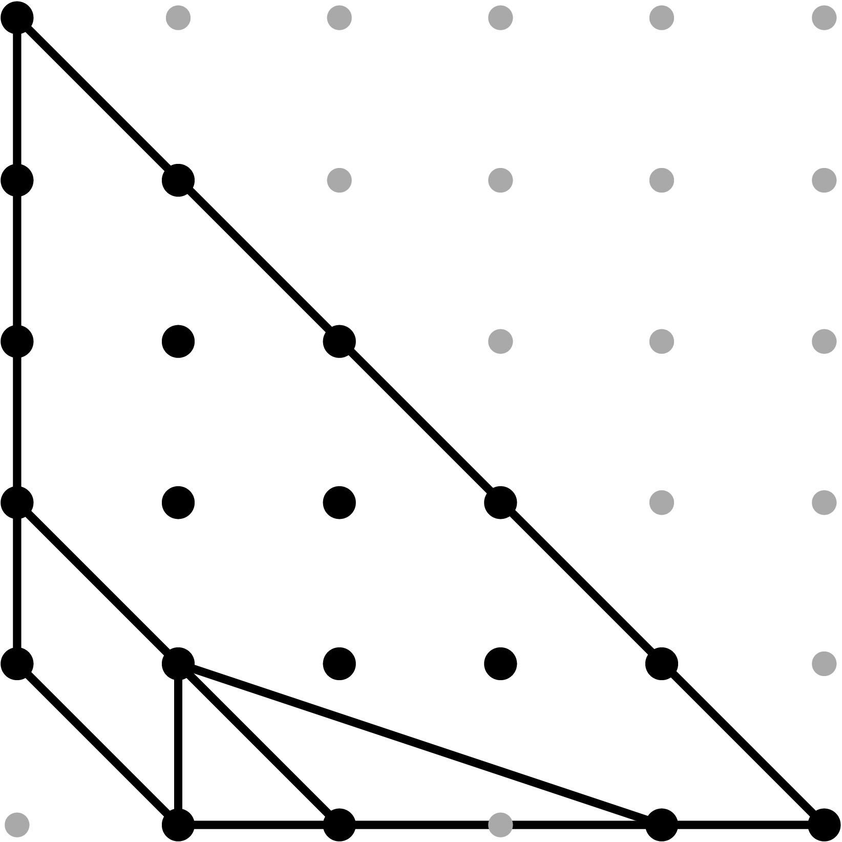
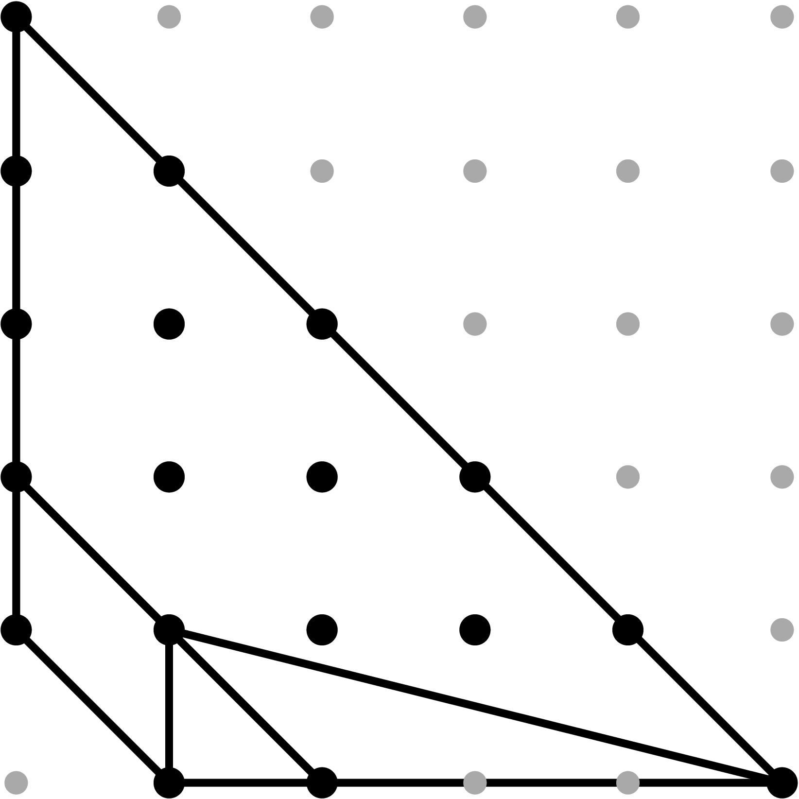
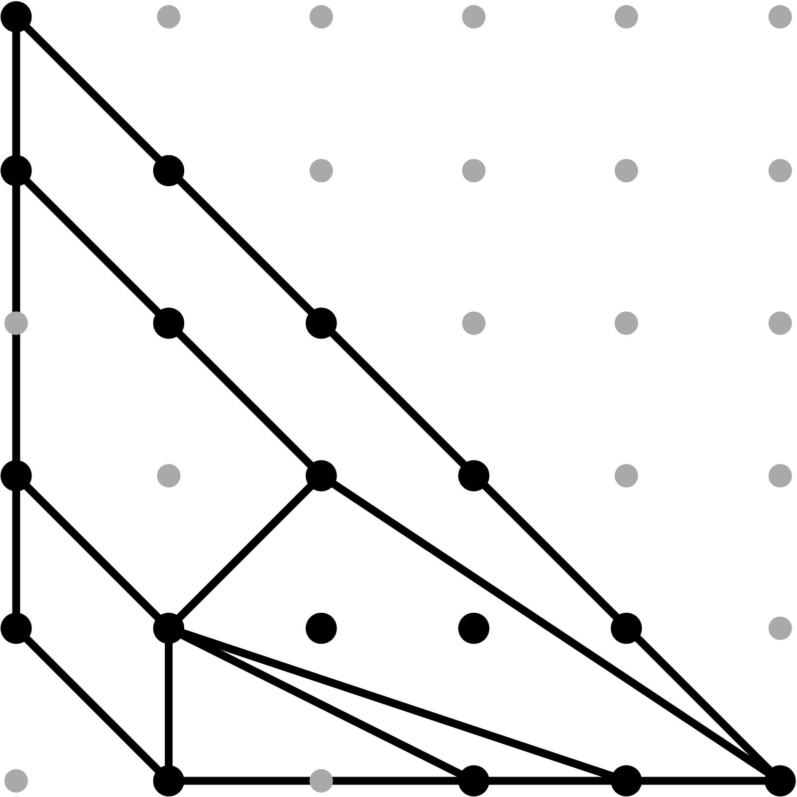
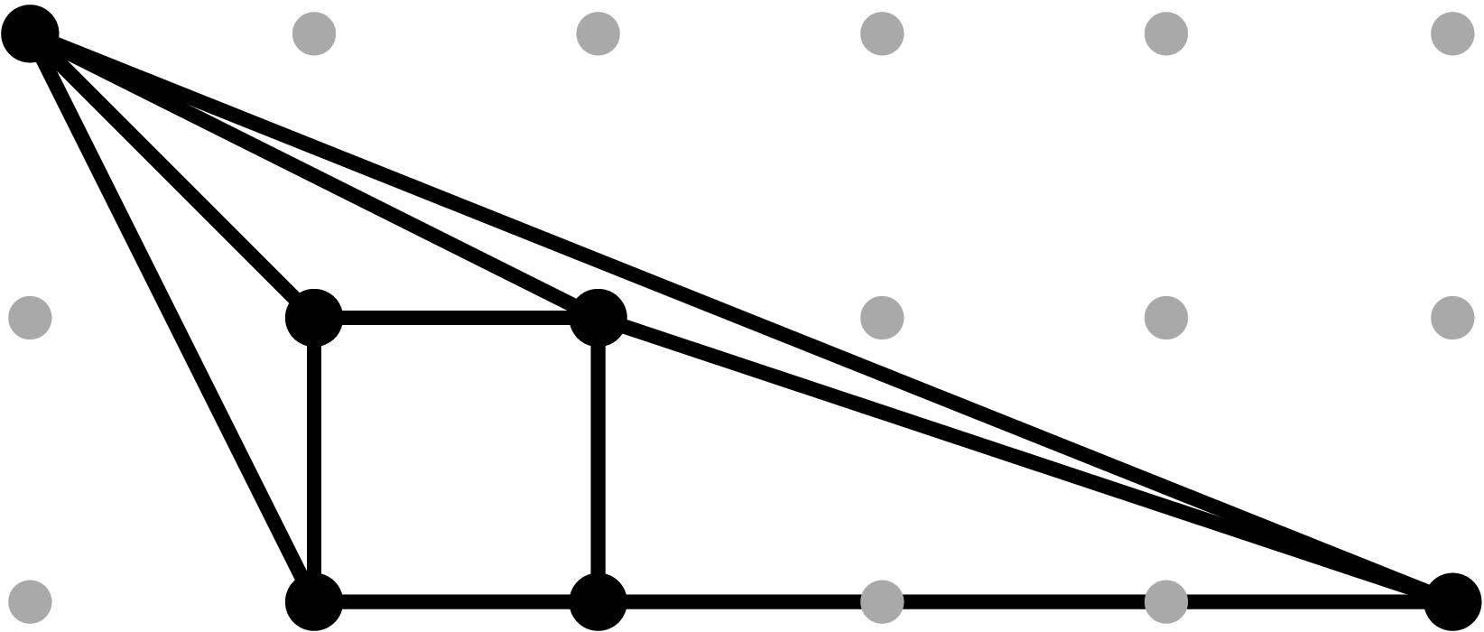
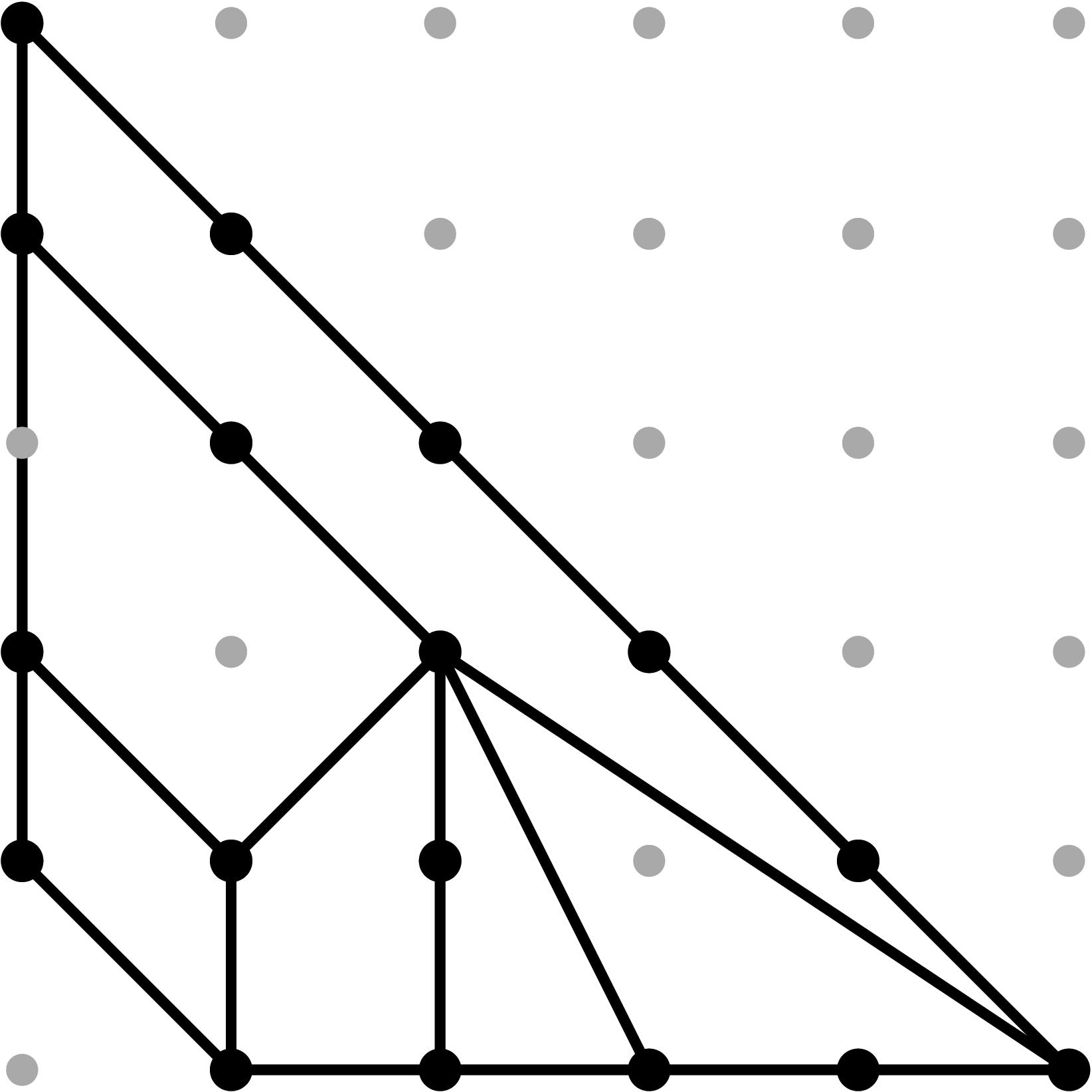
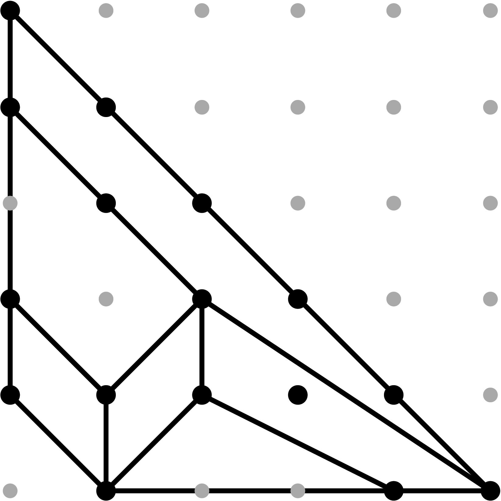
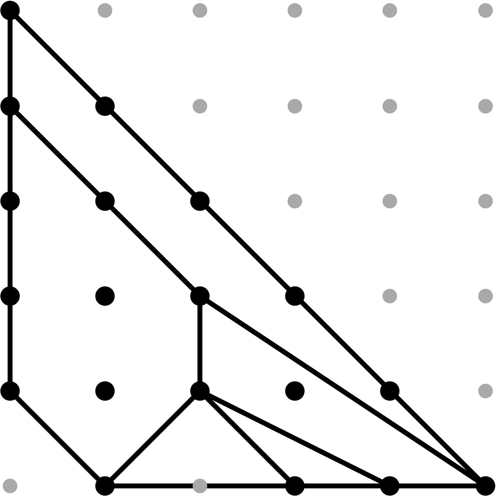
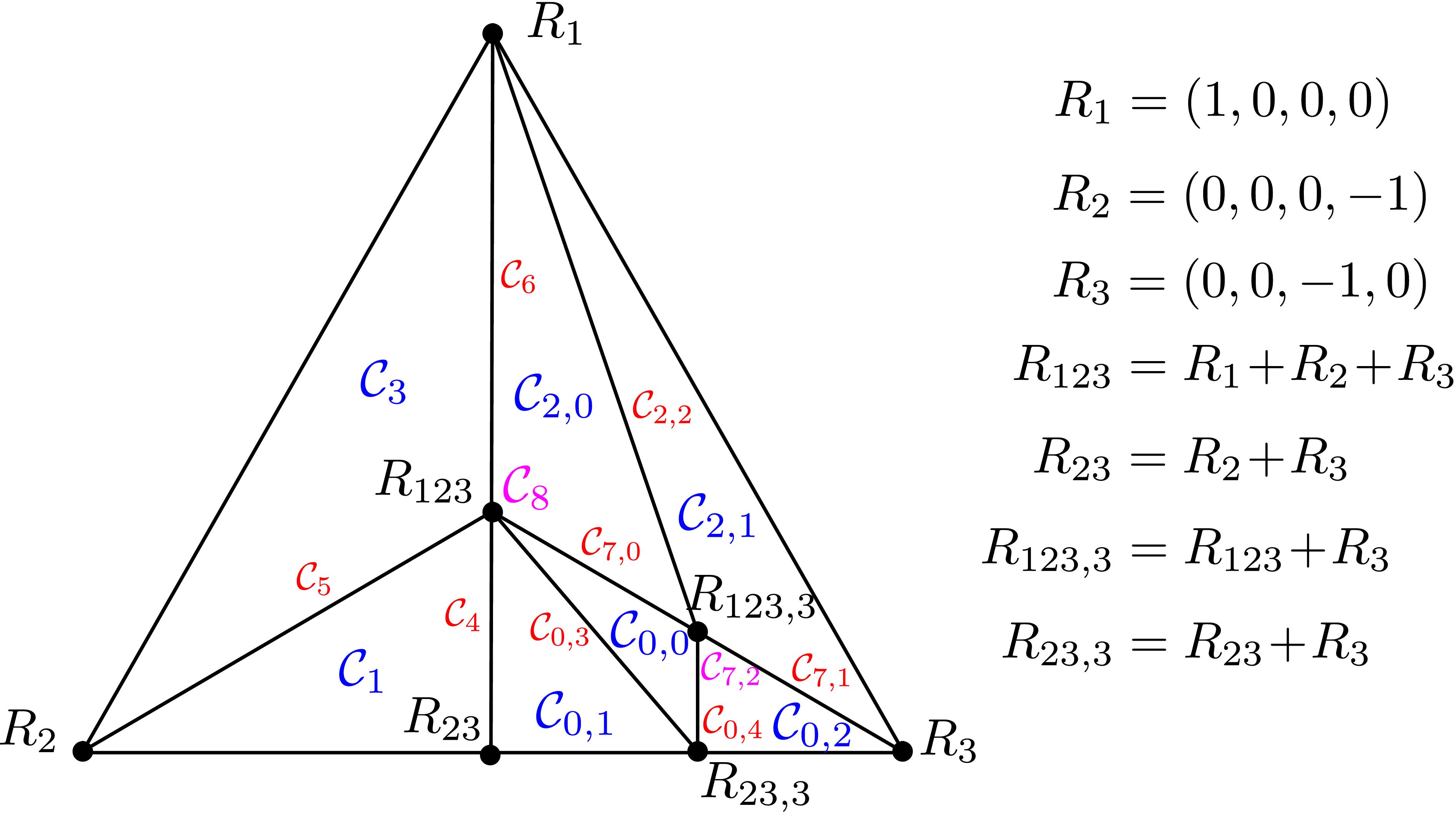Figure 2: Refined subdivision of the Type II Cone induced by all possible Newton subdivisions of the (y,z)-projection. The first index of each cone reflect the label within the subdivision by leading terms of coefficients, as in Figure 1. We use the same color coding for the dimensions of each cone.

Once the refined subdivision and sample points for each piece are computed, we build concrete examples with Puiseux series to determine the Newton subdivisions for each cone assuming the leading terms have the expected valuation. Whenever the leading terms are non-monomial, cancellations of initial terms might occur. The following tables show the combinatorics of each projection and each cone by means of representative examples associated to the chosen sample points, including the relevant Singular scripts and both '.tex' and '.ps' outputs.

Even though the domains of lineality determining the combinatorics of the (y,z)-projection are those given in Figure 2, the combinatorics of the tropicalization induced by the ideal I_g,f agree for most of them. The domains of linealy are given by the subdivision on the left of Figure 1, i.e. the one computed for the (x,z)-projection.

As stated earlier, our branch points are obtained from (b₅,b₄, b₃₄, b₅) via the formulas:

α₂ = b₂² , α₃ = (b₄ + b₃₄)² , α₄ = b₄² and α₂ = - b₅²

The only exception to this rule is provided by the non-generic cases in cells C₄ and C₆ (determined by Tables 1 and 2), where we use α₂ = -b₂². This change turns the non-genericity conditions from in (b₃₄)² = -in (b₂)² to in (b₃₄)² = in (b₂)² (for C₆) and from in (b₄)² = -in (b₂)² to in (b₄)² = in (b₂)² (for C₄). In this way we can construct examples over Q[t] where these genericity conditions are not satisfied.

Jump to:

Cell C_0,0: only generic behavior (Table 0.2.0);
Cell C_0,1: only generic behavior (Table 0.2.1);
Cell C_0,2: only generic behavior (Table 0.2.2);
Cell C_0,3: only generic behavior (Table 0.2.3);
Cell C_0,4: only generic behavior (Table 0.2.4);
Cell C₁: only generic behavior (Table 0.2.5);
Cell C_2,0: only generic behavior (Table 0.2.6);
Cell C_2,1: only generic behavior (Table 0.2.7);
Cell C_2,2: only generic behavior (Table 0.2.8);
Cell C₃: only generic behavior (Table 0.2.9);
Cell C₄: both generic (Table 0.2.10) and non-generic (Table 0.2.11) behavior;
Cell C₅: both generic (Table 0.2.12) and non-generic (Table 0.2.13) behavior;
Cell C₆: both generic (Table 0.2.14) and non-generic (Table 0.2.15) behavior;
Cell C_7,0: both generic (Table 0.2.16) and non-generic (Table 0.2.17) behavior;
Cell C_7,1: both generic (Table 0.2.18) and non-generic (Table 0.2.19) behavior;
Cell C_7,2: both generic (and Table 0.2.20) and non-generic (Table 0.2.21) behavior;
Cell C₈: both generic (and Table 0.2.22) and non-generic behavior;

Cell C_0,0:

**Table 0.2.0: Theta Graph Files and Projections for C_0,0 with sample point [0,-2,-7,-5].**
Parameters	Singular Scripts	(x,y)-subdivision	(x,z)-subdivision	(y,z)-subdivision
b₂ = 3 t⁵ b₃₄ = 5 t⁷ b₄ = 11 t² b₅ = 1+t²	Standard Script (no refinement)	tex output ps output	tex output ps output	tex output ps output

Back to Table of Contents

Cell C_0,1:

**Table 0.2.1: Theta Graph Files and Projections for C_0,1 with sample point [0,-1,-5,-4].**
Parameters	Singular Scripts	(x,y)-subdivision	(x,z)-subdivision	(y,z)-subdivision
b₂ = 3 t⁴ b₃₄ = 5 t⁵ b₄ = 11 t b₅ = 1+t²	Standard Script (no refinement)	tex output ps output	tex output ps output	tex output ps output

Back to Table of Contents

Cell C_0,2:

**Table 0.2.2: Theta Graph Files and Projections for C_0,2 with sample point [0,-1,-6,-3].**
Parameters	Singular Scripts	(x,y)-subdivision	(x,z)-subdivision	(y,z)-subdivision
b₂ = 3 t³ b₃₄ = 5 t⁶ b₄ = 11 t b₅ = 1+t²	Standard Script (no refinement)	tex output ps output	tex output ps output	tex output ps output

Back to Table of Contents

Cell C_0,3:

**Table 0.2.3: Theta Graph Files and Projections for C_0,3 with sample point [0,-1,-4,-3].**
Parameters	Singular Scripts	(x,y)-subdivision	(x,z)-subdivision	(y,z)-subdivision
b₂ = 3 t³ b₃₄ = 5 t⁴ b₄ = 11 t b₅ = 1+t²	Standard Script (no refinement)	tex output ps output	tex output ps output	tex output ps output

Back to Table of Contents

Cell C_0,4:

**Table 0.2.4: Theta Graph Files and Projections for C_0,4 with sample point [0,-1,-5,-3].**
Parameters	Singular Scripts	(x,y)-subdivision	(x,z)-subdivision	(y,z)-subdivision
b₂ = 3 t³ b₃₄ = 5 t⁵ b₄ = 11 t b₅ = 1+t²	Standard Script (no refinement)	tex output ps output	tex output ps output	tex output ps output

Back to Table of Contents

Cell C₁:

**Table 0.2.5: Theta Graph Files and Projections for C₁ with sample point [0,-1,-3,-4].**
Parameters	Singular Scripts	(x,y)-subdivision	(x,z)-subdivision	(y,z)-subdivision
b₂ = 3 t⁴ b₃₄ = 5 t³ b₄ = 11 t b₅ = 1+t²	Standard Script (no refinement)	tex output ps output	tex output ps output	tex output ps output

Back to Table of Contents

Cell C_2,0:

**Table 0.2.6: Theta Graph Files and Projections for C_2,0 with sample point [0,-3,-6,-5].**
Parameters	Singular Scripts	(x,y)-subdivision	(x,z)-subdivision	(y,z)-subdivision
b₂ = 3 t⁵ b₃₄ = 5 t⁶ b₄ = 11 t³ b₅ = 1+t²	Standard Script (no refinement)	tex output ps output	tex output ps output	tex output ps output

Back to Table of Contents

Cell C_2,1:

**Table 0.2.7: Theta Graph Files and Projections for C_2,1 with sample point [0,-2,-5,-3].**
Parameters	Singular Scripts	(x,y)-subdivision	(x,z)-subdivision	(y,z)-subdivision
b₂ = 3 t³ b₃₄ = 5 t⁵ b₄ = 11 t² b₅ = 1+t²	Standard Script (no refinement)	tex output ps output	tex output ps output	tex output ps output

Back to Table of Contents

Cell C_2,2:

**Table 0.2.8: Theta Graph Files and Projections for C_2,2 with sample point [0,-2,-4,-3].**
Parameters	Singular Scripts	(x,y)-subdivision	(x,z)-subdivision	(y,z)-subdivision
b₂ = 3 t³ b₃₄ = 5 t⁴ b₄ = 11 t² b₅ = 1+t²	Standard Script (no refinement)	tex output ps output	tex output ps output	tex output ps output

Back to Table of Contents

Cell C₃:

**Table 0.2.9: Theta Graph Files and Projections for C₃ with sample point [0,-2,-3,-4].**
Parameters	Singular Scripts	(x,y)-subdivision	(x,z)-subdivision	(y,z)-subdivision
b₂ = 5 t⁴ - 17 t⁵ b₃₄ = 7 t³ + 11 t⁹ b₄ = t²+ t⁶ b₅ = 1+t²	Standard Script (no refinement)	tex output ps output	tex output ps output	tex output ps output

Back to Table of Contents

Cell C₄:

In this case, cancellations in the expected initial terms can occur since the relevant leading terms are non-monomial (see Tables 1 and 2). In order to produce cancellations, we need in (b₄)² = -in (b₂)². To avoid computations with complex numbers, we replace b₂ by i b₂, i.e. α₂ = - b₂. With this reparameterization, cancellations will occur if (b₄)² = in (b₂)². As a result, we unmark the point (4,0) from the (y,z)-Newton subdivision. So the unmarked (x,z)-Newton subdivision is unaltered. The resulting plane tropical curves in the generic and special cases agree, as expected.

Table 0.2.10: Theta Graph Files and Projections for Generic C₄ with sample point
[0,-1,-3,-3].
Parameters	Singular Scripts	(x,y)-subdivision	(x,z)-subdivision	(y,z)-subdivision
b₂ = 17 t³ + t⁶ b₃₄ = 5 t³ + t⁹ b₄ = 3 t + t⁷ b₅ = 1+t²	Standard Script (no refinement)	tex output ps output	tex output ps output	tex output ps output

Table 0.2.11: Theta Graph Files and Projections for Special C₄ with sample point
[0,-1,-3,-3].
Parameters	Singular Scripts	(x,y)-subdivision	(x,z)-subdivision	(y,z)-subdivision
b₂ = 5 t³ b₃₄ = 5 t³ b₄ = 3 t + t⁷ b₅ = 1+t²	Standard Script (no refinement)	tex output ps output	tex output ps output	tex output ps output

Back to Table of Contents

Cell C₅:

In this case, cancellations in the expected initial terms can occur since the relevant leading terms are non-monomial (see Tables 1 and 2). In order to produce cancellations in both projections, we need in (b₄)² = in (b₃ b₃₄). If that happens, the point y³ in the (y,z)-projection drops height and we will obtain a potentially subdivided triangle T with vertices (1,0), (4,0) and (1,1) in the (y,z)-Newton subdivision. Two things can occur:

the triangle T is not subdivided;
the triangle is subdivided by the edge yz--y³. For this to occur, we need height(y³)>ω₃ + (ω₅+ω₃+ω₂)/3. We scale our original sample vector by 3, set b₅=1 and add a tail to b₃₄ of the form t ^{- v₃₄+e} for some suitable integer e satisfying the previous height condition. In this case, e=1.

On the (x,z)-projection, the point x³ drops height and we obtain a potentially subdivided triangle T' with vertices (1,0), (4,0) and (1,1) in the (x,y)-Newton subdivision. Two things can occur:

the triangle T' is not subdivided;
the triangle T' is subdivided by the edge xz--x³.

Table 0.2.12: Theta Graph Files and Projections for Generic C₅ with sample point
[0,-1,-2,-3].
Parameters	Singular Scripts	(x,y)-subdivision	(x,z)-subdivision	(y,z)-subdivision
b₂ = 17 t³ + 13 t⁴ b₃₄ = 5 t² - t⁵ b₄ = 3 t + t⁷ b₅ = 1+t²	Standard Script (no refinement)	tex output ps output	tex output ps output	tex output ps output

Table 0.2.13: Theta Graph Files and Projections for Special C₅ with sample points
[0,-1,-2,-3] and [0,-3,-6,-9], respectively.
Parameters	Singular Scripts	(x,y)-subdivision	(x,z)-subdivision	(y,z)-subdivision
b₂ = 17 t³ + 13 t⁴ b₃₄ = 4 t² - t⁵ b₄ = 2 t + t⁷ b₅ = 1+t²	Standard Script (no refinement)	tex output ps output	tex output ps output	tex output ps output
b₂ = 17 t⁹ + 13 t¹² b₃₄ = 4 t⁶ - t⁷ b₄ = 2 t³ b₅ = 1	Standard Script (no refinement)	tex output ps output	tex output ps output	tex output ps output

Back to Table of Contents

Cell C₆:

In this case, cancellations in the expected initial terms can occur since the relevant leading terms are non-monomial (see Tables 1 and 2). In order to produce cancellations, we need in (b₃₄)² = -in (b₂)². To avoid computations with complex numbers, we replace b₂ by i b₂, i.e. α₂ = - b₂. With this reparameterization, cancellations will occur if (b₃₄)² = in (b₂)². If that happens, the point y³ drops height in the (y,z)-projection and we will obtain a potentially subdivided triangle T with vertices (2,0), (5,0) and (2,2) in the (y,z)-Newton subdivision. Two things can occur:

the triangle T is not subdivided;
the triangle T is subdivided by the edge y² z² -- y³. For this to occur, we need height(y³) > 2 (ω₅+ω₄+ω₂)/3. We scale our original sample vector by 3, set b₂=t^-ω₂/2 and add a tail to b₃₄ of the form t ^{- v₃₄+e} for some suitable integer e satisfying the previous height condition. In this case, e=1.

On the (x,z)-projection, the point x³ drops height and we obtain a potentially subdivided triangle T' with vertices (2,0), (5,0) and (2,1) in the (x,y)-Newton subdivision. Two things can occur:

the triangle T' is not subdivided;
the triangle T' is subdivided by the edge x² z -- x³.

Table 0.2.14: Theta Graph Files and Projections for Generic C₆ with sample point
[0,-2,-3,-3].
Parameters	Singular Scripts	(x,y)-subdivision	(x,z)-subdivision	(y,z)-subdivision
b₂ = 17 t³ + t⁶ b₃₄ = 5 t³ + t¹⁰ b₄ = 4 t² + t⁵ b₅ = 1+t²	Standard Script (no refinement)	tex output ps output	tex output ps output	tex output ps output

Table 0.2.15: Theta Graph Files and Projections for Special C₆ with sample points
[0,-2,-3,-3] and [0,-6,-9,-9], respectively.
Parameters	Singular Scripts	(x,y)-subdivision	(x,z)-subdivision	(y,z)-subdivision
b₂ = t³ + t⁶ b₃₄ = t³ + t¹⁰ b₄ = 4 t² + t⁵ b₅ = 1+t²	Standard Script (no refinement)	tex output ps output	tex output ps output	tex output ps output
b₂ = t⁹ b₃₄ = t⁹ + t¹⁰ b₄ = t⁶ + t¹⁵ b₅ = 1 + t⁶	Standard Script (no refinement)	tex output ps output	tex output ps output	tex output ps output

Back to Table of Contents

Cell C_7,0:

In this case, cancellations in the expected initial terms can occur since the relevant leading terms are non-monomial (see Tables 1 and 2). In order to produce cancellations in both projections, we need in (b₄)² = in (b₂ b₅). If that happens, the point y³ in the (y,z)-projection drops height and we will obtain a potentially subdivided triangle T with vertices (1,0), (4,0) and (1,1). Two things can occur:

the triangle T is not subdivided;
the triangle T is subdivided by the edge yz--y³. For this to occur, we need height(y³)> 2 d₃₄/3 + ω₂ + ω₃ + 7 ω₅/3. We scale our original sample vector by 3, set b₅=1 and add a tail to b₂ of the form t ^{- ω₂/2 + e} for some suitable integer e satisfying the previous height condition. In this case, e=1.

On the (x,z)-projection, the point x³ becomes unmarked and we obtain a trapezoid with vertices (1,0), (5,0), (2,1) and (1,1) that cannot be further subdivided.

Table 0.2.16: Theta Graph Files and Projections for Generic C_7,0 with sample point
[0,-2,-5,-4].
Parameters	Singular Scripts	(x,y)-subdivision	(x,z)-subdivision	(y,z)-subdivision
b₂ = 3 t⁴ b₃₄ = 5 t⁵ b₄ = 11 t² b₅ = 1+t²	Standard Script (no refinement)	tex output ps output	tex output ps output	tex output ps output

Table 0.2.17: Theta Graph Files and Projections for Special C_7,0 with sample points
[0,-2,-5,-4] and [0,-6,-15,-12], respectively.
Parameters	Singular Scripts	(x,y)-subdivision	(x,z)-subdivision	(y,z)-subdivision
b₂ = 4 t⁴ + t¹⁶ b₃₄ = t⁵ + t¹⁰ b₄ = 2 t² + t⁵ b₅ = 1 + t²	Standard Script (no refinement)	tex output ps output	tex output ps output	tex output ps output
b₂ = 4 t¹² + t¹³ b₃₄ = t¹⁵ b₄ = 2 t⁶ b₅ = 1	Standard Script (no refinement)	tex output ps output	tex output ps output	tex output ps output

Back to Table of Contents

Cell C_7,1:

In this case, cancellations in the expected initial terms can occur since the relevant leading terms are non-monomial (see Tables 1 and 2). In order to produce cancellations in both projections, we need in (b₄)² = in (b₂ b₅). If that happens, the point y³ in the (y,z)-projection drops height and we will obtain a potentially subdivided triangle T with vertices (1,0), (4,0) and (1,1). Two things can occur:

the triangle T is not subdivided;
the triangle T is subdivided by the edge yz--y³. For this to occur, we need height(y³)> 2 d₃₄/3 + ω₂ + ω₃ + 7 ω₅/3. We add a tail to b₂ of the form t ^{- ω₂/2 + e} for some suitable integer e satisfying the previous height condition. In this case, e=1.

On the (x,z)-projection, the point x³ becomes unmarked and we obtain a trapezoid with vertices (1,0), (5,0), (2,1) and (1,1) that cannot be further subdivided.

Table 0.2.18: Theta Graph Files and Projections for Generic C_7,1 with sample point
[0,-1,-4,-2].
Parameters	Singular Scripts	(x,y)-subdivision	(x,z)-subdivision	(y,z)-subdivision
b₂ = 3 t² b₃₄ = 5 t⁴ b₄ = 11 t b₅ = 1+t²	Standard Script (no refinement)	tex output ps output	tex output ps output	tex output ps output

Table 0.2.19: Theta Graph Files and Projections for Special C_7,1 with sample point
[0,-1,-4,-2].
Parameters	Singular Scripts	(x,y)-subdivision	(x,z)-subdivision	(y,z)-subdivision
b₂ = 4 t² + t¹⁶ b₃₄ = t⁴ + t¹⁰ b₄ = 2 t + t⁵ b₅ = 1 + t²	Standard Script (no refinement)	tex output ps output	tex output ps output	tex output ps output
b₂ = 4 t² + t³ b₃₄ = t⁴ b₄ = 2 t b₅ = 1	Standard Script (no refinement)	tex output ps output	tex output ps output	tex output ps output

Back to Table of Contents

Cell C_7,2:

In this case, cancellations in the expected initial terms can occur since the relevant leading terms are non-monomial (see Tables 1 and 2). In order to produce cancellations in both projections, we need in (b₄)² = in (b₂ b₅). If that happens, the point y³ in the (y,z)-projection drops in height and we obtain a potentially subdivided triangle T with vertices (1,0), (4,0) and (1,1). Two things can occur:

the triangle T is not subdivided;
the triangle T is subdivided by the edge yz--y³. For this to occur, we need height(y³)> 2 d₃₄/3 + ω₂ + ω₃ + 7 ω₅/3. We scale our original sample vector by 3, set b₅=1 and add a tail to b₂ of the form t ^{- ω₂/2 + e} for some suitable integer e satisfying the previous height condition. In this case, e=1.

On the (x,z)-projection, the point x³ becomes unmarked and we obtain a trapezoid with vertices (1,0), (5,0), (2,1) and (1,1) that cannot be further subdivided.

Table 0.2.20: Theta Graph Files and Projections for Generic C_7,2 with sample point
[0,-1,-3,-2].
Parameters	Singular Scripts	(x,y)-subdivision	(x,z)-subdivision	(y,z)-subdivision
b₂ = 3 t² b₃₄ = 5 t³ b₄ = 11 t b₅ = 1+t²	Standard Script (no refinement)	tex output ps output	tex output ps output	tex output ps output

Table 0.2.21: Theta Graph Files and Projections for Special C_7,2 with sample points
[0,-1,-3,-2] and [0,-3,-9,-6], respectively.
Parameters	Singular Scripts	(x,y)-subdivision	(x,z)-subdivision	(y,z)-subdivision
b₂ = 4 t² b₃₄ = t³ b₄ = 2 t b₅ = 1 + t²	Standard Script (no refinement)	tex output ps output	tex output ps output	tex output ps output
b₂ = 4 t⁶ + t⁷ b₃₄ = t⁹ b₄ = 2 t³ b₅ = 1	Standard Script (no refinement)	tex output ps output	tex output ps output	tex output ps output

Back to Table of Contents

Cell C₈:

In this case, cancellations in the expected initial terms can occur since the relevant leading terms are non-monomial (see Tables 1 and 2). Depending on our choice of factors to cancel (determined by Tables 1 and 2), the effect of cancellations will be to unmark the points y² z or y³ and/or y⁴ on the (y,z)-Newton subdivision and unmark x³ on the (x,z)-Newton subdivision. This has no impact on the tropical world, so we omit including an example.

Table 0.2.22: Theta Graph Files and Projections for Generic C₈ with sample point
[0,-1,-2,-2].
Parameters	Singular Scripts	(x,y)-subdivision	(x,z)-subdivision	(y,z)-subdivision
b₂ = 17 t² + t⁶ b₃₄ = 5 t² + t¹⁰ b₄ = 4 t + t⁵ b₅ = 1+t²	Standard Script (no refinement)	tex output ps output	tex output ps output	tex output ps output

Back to Table of Contents

§0.3 Type (III) Cone (Figure Eight):

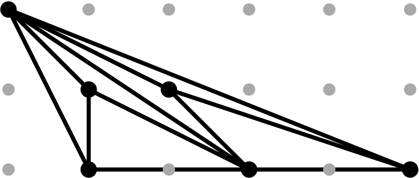
In addition to the modification along F and its lifting f, we compute a vertical modification along MAX{X,ω₄} with lifting u = x - α₄. This produces a faithful tropicalization at the level of the extended skeleta. We recover the resulting tropical curve in R⁴ by means of the planar (x,y), (x,z), (u,y) and (u,z)-projections.

**Table 0.3: Figure Eight Graph Files and Projections.**
Branch points	Singular Scripts	(x,y)-subdivision	(x,z)-subdivision	(u,y)-subdivision	(u,z)-subdivision	(y,z)-subdivision
α₂ = (t⁹+t¹²)² α₃ = (t⁵+t⁹)² α₄ = (3 t⁵+t⁸)² α₅ = -(1+t⁵)²	Standard Script (no refinement)	tex output ps output	tex output ps output	tex output ps output	tex output ps output	tex output ps output
α₂ = (t⁹+t¹²)² α₃ = (t⁵+t⁹)² α₄ = (3 t⁵+t⁸)² α₅ = -(1+t⁵)²	Refinement Script (t^ε and t^ε') ε = 3 ε'= 4	tex output ps output	tex output ps output	tex output ps output	tex output ps output	tex output ps output

§0.4 Type (IV) Cone:

The following files are used to compute the negative valuation of the j-invariant of the curve dual to the genus 1 vertex on the xy-projection.

Singular Script to compute the j-invariant of the curve. [Plain text output]
Sage file containg the input numerator and denominator of the j-invariant (the file is in plain text).
Sage script of auxiliary functions for Gröbner fan computations, subdivisions of cones induced by Gröbner fans, leading terms with respect to weight vectors.
Sage script that computes the leading term (by our own implementation and by generating a script to run in Macaulay 2) of both the numerator and denominator of the j-invariant, factors the resulting forms and checks the Type (VI) Cone lies in a single cone of both the numerator and denominator of the j-invariant.
Macaulay 2 file that computes the leading terms of both the numerator and denominator of the j-invariant. The output of the computation is commented within the file.
Sage script that computes the Gröbner cones of the numerator and denominator of the j-invariant. The file records the f-vector, rays and maximal cones. [Compressed output of the Gröbner fan and its maximal cones]

**Table 0.4: Type IV Graph Files and Projections.**
Branch points	Singular Scripts	(x,y)-subdivision	(x,z)-subdivision	(u,y)-subdivision	(u,z)-subdivision	(y,z)-subdivision
α₂ = (t¹⁴+t¹⁶)² α₃ = (t⁵+t⁹)² α₄ = (3 +t⁸)² α₅ = - (1+t⁵)²	Standard Script (no refinement)	tex output ps output	tex output ps output	tex output ps output	tex output ps output	tex output ps output
α₂ = (t¹⁴+t¹⁶)² α₃ = (t⁵+t⁹)² α₄ = (3 +t⁸)² α₅ = - (1+t⁵)²	Refinement Script (t^ε only) ε = 8	tex output ps output	tex output ps output	tex output ps output	tex output ps output	tex output ps output

§0.5 Type (V) Cone:

The following files are used to compute the negative valuation of the j-invariant of the curves dual to each of the genus 1 vertices on the xy-projection.

Singular Script to compute the j-invariant of the curves. [Plain text output of the rightmost vertex]. [Plain text output of the leftmost vertex]
Sage file containg the input numerator and denominator of the j-invariant of the leftmost vertex (the file is in plain text).
Sage file containg the input numerator and denominator of the j-invariant of the rightmost vertex (the file is in plain text).
Sage script of auxiliary functions for Gröbner fan computations, subdivisions of cones induced by Gröbner fans, leading terms with respect to weight vectors.
Sage script that computes the leading term (by our own implementation and by generating a script to run in Macaulay 2) of both the numerator and denominator of the two j-invariants, factors the resulting forms and checks the Type (V) Cone lies in a single cone of both the numerator and denominator of the two j-invariant.
Macaulay 2 file that computes the leading terms of both the numerator and denominator of the j-invariant of the leftmost vertex. The output of the computation is commented within the file.
Macaulay 2 file that computes the leading terms of both the numerator and denominator of the j-invariant of the rightmost vertex. The output of the computation is commented within the file.
Sage script that computes the Gröbner cones of the numerator and denominator of the j-invariant of the leftmost vertex. The file records the f-vector, rays and maximal cones. [Compressed output of the Gröbner fan and its maximal cones]
Sage script that computes the Gröbner cones of the numerator and denominator of the j-invariant of the rightmost vertex. The file records the f-vector, rays and maximal cones. [Compressed output of the Gröbner fan and its maximal cones]

If we compute two successive vertical modifications along MAX{X,ω₄} and MAX{X,ω₂} (in that order), with liftings z₂ = x - α₂, and z₄ = x - α₄, we produce a faithful tropicalization at the level of the extended skeleta. We can compute the resulting tropical curve in R⁴ by means of the planar (x,y), (z₂,y) and (z₄,y)-projections.

**Table 0.5: Type V Graph Files and Projections associated to two vertical modifications.**
Branch points	Singular Scripts	(x,y)-subdivision	(z₂,y)-subdivision	(z₄,y)-subdivision
α₂ = (5 t¹⁴+t¹⁶)² α₃ = (t¹⁴+t¹⁹)² α₄ = (3 +t⁸)² α₅ = - (1+t⁵)²	Standard Script (no refinement)	tex output ps output	tex output ps output	tex output ps output

§0.6 Type (VI) Cone:

There are several possibilities for the (x,z)-projection, depending on the genericity of the initial forms of α₃, α₄, α₅, β₃ and β₄ with respect to the expected coefficients for x³ and x⁴.

Genericity for x⁴: in(α₃) + in(α₄) ≠ 0,
Genericity for x³: in(α₅) (in(β₃) - in(β₄))² + in(α₃) in(α₄) ≠ 0.

Generic for x³ (any condition for x⁴):

In addition to the modification along F and its lifting f, we compute two successive vertical modifications along MAX{X,ω₄}, with liftings z₃ = x - α₃, and z₄ = x - α₄. This produces a faithful tropicalization at the level of the extended skeleta. We recover the resulting tropical curve in R⁵ by means of the planar (x,y), (z₃,y) and (z₄,y)-projections. Notice that the the last two agree with the (z₄,y) and (z₄,z)-projections so the latter ones need not be plotted.

**Table 0.6.0: Type VI Graph Files and Projections in the generic case for x³.**
Branch points	Singular Scripts	(x,y)-subdivision	(x,z)-subdivision	(z₃,y)- and (z₄,y)-subdivisions	(z₃,z)- and (z₄,z)-subdivision	(y,z)-subdivision
α₂=(t¹⁴+t¹⁶)² α₃= (5+t⁹)² α₄= (3 +t⁸)² α₅= - (1+t⁵)²	Standard Script (no ref.)	tex output ps output	tex output ps output	tex output (z₃y) ps output (z₃y) tex output (z₄y) ps output (z₄y)	tex output (z₃z) ps output (z₃z) tex output (z₄z) ps output (z₄z)	tex output ps output
α₂=(t¹⁴+t¹⁶)² α₃= (5+t⁹)² α₄= (3 +t⁸)² α₅= - (1+t⁵)²	Refinement Script (t^ε only) ε = 13	tex output ps output	tex output ps output	tex output (z₃y) ps output (z₃y) tex output (z₄y) ps output (z₄y)	tex output (z₃z) ps output (z₃z) tex output (z₄z) ps output (z₄z)	tex output ps output

Generic for x⁴, Non-Generic for x³ but x³ marked:

In addition to the modification along F and its lifting f, we compute two successive vertical modifications along MAX{X,ω₄}, with liftings z₃ = x - α₃, and z₄ = x - α₄. This produces a faithful tropicalization at the level of the extended skeleta. We recover the resulting tropical curve in R⁵ by means of the planar (x,y), (z₃,y) and (z₃,z)-projections. Notice that the the last two agree with the (z₄,y) and (z₄,z)-projections so the latter ones need not be plotted.

**Table 0.6.1: Type VI Graph Files and Projections in the non-generic case for x³ but x³ marked.**
Branch points	Singular Scripts	(x,y)-subdivision	(x,z)-subdivision	(z₃,y)- and (z₄,y)-subdivisions	(z₃,z)- and (z₄,z)-subdivision	(y,z)-subdivision
α₂=(t¹⁴+t¹⁶)² α₃= (2+t⁹)² α₄= (1 +t⁸)² α₅= - (2+t⁵)²	Standard Script (no ref.)	tex output ps output	tex output ps output	tex output (z₃y) ps output (z₃y) tex output (z₄y) ps output (z₄y)	tex output (z₃z) ps output (z₃z) tex output (z₄z) ps output (z₄z)	tex output ps output
α₂=(t¹⁴+t¹⁶)² α₃= (5+t⁹)² α₄= (3 +t⁸)² α₅= - (1+t⁵)²	Refinement Script (t^ε only) ε = 13	tex output ps output	tex output ps output	tex output (z₃y) ps output (z₃y) tex output (z₄y) ps output (z₄y)	tex output (z₃z) ps output (z₃z) tex output (z₄z) ps output (z₄z)	tex output ps output

Generic for x⁴, Non-Generic for x³ and x³ unmarked:

In addition to the modification along F and its lifting f, we compute two successive vertical modifications along MAX{X,ω₄}, with liftings z₃ = x - α₃, and z₄ = x - α₄. This produces a faithful tropicalization at the level of the extended skeleta. We recover the resulting tropical curve in R⁵ by means of the planar (x,y), (z₃,y) and (z₃,z)-projections. Notice that the the last two agree with the (z₄,y) and (z₄,z)-projections so the latter ones need not be plotted.

**Table 0.6.2: Type VI Graph Files and Projections in the non-generic case for x³ and x³ unmarked.**
Branch points	Singular Scripts	(x,y)-subdivision	(x,z)-subdivision	(z₃,y)- and (z₄,y)-subdivisions	(z₃,z)- and (z₄,z)-subdivision	(y,z)-subdivision
α₂=(t¹⁴+t¹⁶)² α₃= (2)² α₄= (1)² α₅= - (2)²	Standard Script (no ref.)	tex output ps output	tex output ps output	tex output (z₃y) ps output (z₃y) tex output (z₄y) ps output (z₄y)	tex output (z₃z) ps output (z₃z) tex output (z₄z) ps output (z₄z)	tex output ps output
α₂=(t¹⁴+t¹⁶)² α₃= (2)² α₄= (1)² α₅= - (2)²	Refinement Script (t^ε only) ε = 13	tex output ps output	tex output ps output	tex output (z₃y) ps output (z₃y) tex output (z₄y) ps output (z₄y)	tex output (z₃z) ps output (z₃z) tex output (z₄z) ps output (z₄z)	tex output ps output

Non-Generic for x⁴ and also for x³:

Recall that

α₂=β₂², α₃= β₃², α₄= β₄² and α₅= - β₅².

Violating The genericity conditions for both x³ and x⁴ requires the use of non-real numbers, since we must have

(in (β₃))² = in (α₃) = -in(α₄) = - ( in (β₄))² and in (β₃) in (β₄) = in (β₅) (in (β₃) - in (β₄)).

We take in (β₅) = 1, in (β₃) = (ι - 1), and in (β₄) = (1 + ι). We produce all the numerical examples by evaluating all the elimination ideals at the desired values of β₂, β₃, β₄, and β₅ with Singular, by working with the field extension associated to the polynomial x² + 1. To plot the tropical plane curves with Singular, we replace each polynomial by one with coefficients in Q[t] with the same t-valuation (the result is obtained by specializing the Symbolic computations to a random value of ι.) As was mentioned, we only treat the refined modifications.

**Table 0.6.3: Type VI Graph Files and Projections in the non-generic case for x³ and x⁴ for refined modifications.**
Branch points	Singular Scripts	(x,y)-subdivision	(x,z)-subdivision	(z₃,y)- and (z₄,y)-subdivisions	(z₃,z)- and (z₄,z)-subdivision	(y,z)-subdivision
α₂=(5t¹⁴+t¹⁶)² α₃=(ι-1+t¹⁸)² α₄= (1+ι)² α₅= - 1	Refinement Script with Symbolic ι Refinement Script with Numerical ι (t^ε and t^ε') ε = 1 ε' = 2	tex output ps output	tex output ps output	tex output (z₃y) ps output (z₃y) tex output (z₄y) ps output (z₄y)	tex output (z₃z) ps output (z₃z) tex output (z₄z) ps output (z₄z)	tex output ps output

§0.7 Type (VII) Cone (Good Reduction):

If we compute three successive vertical modifications along MAX{X,ω₂} with 3 different liftings

z₂ = x - α₂, z₃ = x - α₃, and z₄ = x - α₄,

we produce a faithful tropicalization at the level of the extended skeleta. We can compute the resulting tropical curve in R⁵ by means of the planar (x,y), (z₂,y), (z₃,y), and (z₄,y)-projections. Notice that these 3 projections are indistinguishable. Their sole purpose is to isolate the leg marked by the corresponding branch point.

**Table 0.7.1: Type VII Graph Files and Projections associated to three vertical modifications.**
Branch points	Singular Scripts	(x,y)-subdivision	(z₂,y)-subdivision	(z₃,y)-subdivision	(z₄,y)-subdivision
α₂ = ( t¹⁰+t¹²)² α₃ = (4 t¹⁰+t¹⁹)² α₄ = (3 t¹⁰+t¹⁸)² α₅ = - (12 t¹⁰)²	Standard Script (no refinement)	tex output ps output	tex output ps output	tex output ps output	tex output ps output

§1. Igusa invariants and their tropicalizations

The following scripts allow to compute initial forms of the corresponding polynomials A, B, C, A', B', C', Q₃ = AB - 3C, Q₄ = AB - 4C, and Q₄' = A'B' - 4C'. We refer to the last two sections of the paper for the definition of these polynomials.

The variables for A, B, C, Q₃ and Q₄ are ordered as the tuple x = (a₆, a₅, a₄, a₃, a₂, a₁).
The variables for A', B', C', and Q₄' are ordered as the tuple x = (a₆, a₅, x₃₄, a₃, a₂, a₁).
Sage script generating the polynomials A, B, C, A', B', C', Q₃, Q₄ and Q₄', and the M2 scripts to compute the initial forms with respect to weights in the Dumbbell and Theta Cone. In addition, it computes the Gröbner fan of Q₄' and the subdivision induced on the Theta cone.
Sage script generating all 7 polyhedral cones representing the 7 cells in M₂^trop and sample points on each cone. We use the variables (a₆, a₅, x₃₄, a₃, a₂, a₁) only for the Theta Cone.
Sage script that computes the Gröbner cones of the polynomials A and A' and computes the subdivision on all 7 cones in M₂^trop induced by these fans. The file records the f-vector, rays and maximal cones and verifies that no subdivision is performed. We save the output fans as Sage objects. [Output for A] [Output for A']
Sage script that computes the Gröbner cones of the polynomials B and B' and computes the subdivision on all 7 cones in M₂^trop induced by these fans. The file records the f-vector, rays and maximal cones and verifies that no subdivision is performed. We save the output fans as Sage objects. [Output for B] [Output for B']
Sage script that computes the Gröbner cones of the polynomials C and C' and computes the subdivision on all 7 cones in M₂^trop induced by these fans. The file records the f-vector, rays and maximal cones and verifies that no subdivision occurs. We save the output fans as Sage objects. [Output for C] [Output for C']
Sage script that computes the Gröbner cones of the polynomials Q₄ and Q₄' and computes the subdivision on all 7 cones in M₂^trop induced by these fans. The file records the f-vector, rays and maximal cones and verifies that the only subdivision produced is in the Theta cone. We save the output fans as Sage objects. [Output for Q₄] [Output for Q₄']

We separate the Macaulay2 scripts into two types, depending on the maximal cone in M₂^trop. We assume the characteristic of the residue field to be different than 2 and 3. Our own implementation of the leading terms is given at the end of this section, and includes the computation for all lower dimensional cones.

§1.1 Dumbbell Cone

In all our scripts we input a weight vector ω=(ω₆,ω₅,ω₄,ω₃,ω₂,ω₁) in R⁶, where -val(α_i) = ω_i for i=1,…, 6. The vector ω lies in the Dumbbell cone since it satisfies:

ω₁ < ω₂ < ω₃ < ω₄ < ω₅ < ω₆

In all the scripts below, we fix ω = (36,25,20,16,9,1). The scrpts where generated from the Sage script provided above. The outputs of the computations are commented after each command in the scripts.

Macaulay 2 Script computating the initial form of A with respect to the weight vector ω;
Macaulay 2 Script computating the initial form of B with respect to the weight vector ω;
Macaulay 2 Script computating the initial form of C with respect to the weight vector ω;
Macaulay 2 Script computating the initial form of Q₃ = A B - 3 C with respect to the weight vector ω;
Macaulay 2 Script computating the initial form of Q₄ = A B - 4 C with respect to the weight vector ω;
Macaulay 2 Script computating the initial form of A, B, C, Q₃ and Q₄ with respect to the weight vector ω.

§1.2 Theta Cone

In all our scripts we input a weight vector ω=(ω₆,ω₅,d₃₄,ω₃,ω₂,ω₁) in R⁶, where -val(α_i) = ω_i for i=1,2,3, 5, 6, and -val(x₃₄) = d₃₄. Recall that x₃₄ = α₄ - α₃.

The vector ω lies in the Theta cone since it satisfies:

ω₁ < ω₂ < ω₃ <ω₅ < ω₆ and d₃₄ < ω₃.

The Sage script at the begining of this section computes the Gröbner fan of Q₄' = A'B' - 4 C' by replacing Q₄' by the sum of its extremal monomials. Its f-vector equals [1, 32, 174, 396, 420, 168].

Sage Object: Gröbner fan of Q₄' in R⁶ given as a polyhedral fan data type.
Sage Object: Gröbner fan of Q₄' in R⁶ given as a rational polyhedral fan data type. This file is used to subdivide the Theta cone.

The calculation yields a subdivision of the Theta cone into 3 pieces, which we call Θ₀, Θ₁ and Θ₂. The Sage calculation gives the inequalities and extremal rays for each piece, recorded in Table 2 below. We compute a sample point on the relative interior of each piece by adding up the extremal rays and translating by the all ones vector to get non-negative weights for each variable. The variables are ordered as the tuple x = (a₆, a₅, x₃₄, a₃, a₂, a₁).

**Table 2: Combinatorial data of the Subdivision of the Theta cone induced by the Gröbner fan of Q₄'.**
Cell	Defining inequalities	Extremal rays	Lines	Sample point
Θ₀	(0, 0, -1, 1, 0, 0) x + 0 >= 0, (0, 0, 0, 0, 1, -1) x + 0 >= 0, (1, -1, 0, 0, 0, 0) x + 0 >= 0, (0, 0, 1, 0, -1, 0) x + 0 >= 0, (0, 1, 1, -2, 0, 0) x + 0 >= 0	(0, 0, 0, 0, 0, -1) (0, 0, 0, 0, -1, -1) (0, 0, -2, -1, -2, -2) (0, 0, -1, -1, -1, -1) (0, -1, -1, -1, -1, -1)	(1, 1, 1, 1, 1, 1)	ω⁽⁰⁾=(6, 5, 2, 3, 1, 0);
Θ₁	(0, -1, -1, 2, 0, 0) x + 0 >= 0, (0, -1, 0, 2, -1, 0) x + 0 >= 0, (1, -1, 0, 0, 0, 0) x + 0 >= 0, (0, 1, 0, -1, 0, 0) x + 0 >= 0, (0, 0, 0, 0, 1, -1) x + 0 >= 0	(0, -1, -1, -1, -1, -1) (0, 0, 0, 0, 0, -1) (0, 0, 0, 0, -1, -1) (0, 0, -1, 0, 0, 0) (0, 0, -2, -1, -2, -2)	(1, 1, 1, 1, 1, 1)	ω⁽¹⁾=(6, 5, 2, 4, 2, 1);
Θ₂	(0, 0, -1, 0, 1, 0) x + 0 >= 0, (1, -1, 0, 0, 0, 0) x + 0 >= 0, (0, 0, 0, 0, 1, -1) x + 0 >= 0, (0, 0, 0, 1, -1, 0) x + 0 >= 0, (0, 1, 0, -2, 1, 0) x + 0 >= 0	(0, 0, 0, 0, 0, -1) (0, 0, -1, 0, 0, 0) (0, 0, -2, -1, -2, -2) (0, -1, -1, -1, -1, -1) (0, 0, -1, -1, -1, -1)	(1, 1, 1, 1, 1, 1)	ω⁽²⁾=(6, 5, 1, 3, 2, 1)

Macaulay2 scripts to confirm the calculation of the initial forms on the three pieces of the Theta cone. The outputs of the computations are commented after each command in the scripts. The calculations are also done at the end of the Sage script by computing the leading terms as the monomials maximizing the inner product between the weight vector and the exponent vectors.

Macaulay 2 Script computating the initial form of A, B, C, Q₄' with respect to the weight vector ω⁽⁰⁾ = (6, 5, 2, 3, 1, 0);
Macaulay 2 Script computating the initial form of A, B, C, Q₄' with respect to the weight vector ω⁽¹⁾=(6, 5, 2, 4, 2, 1);
Macaulay 2 Script computating the initial form of A, B, C, Q₄' with respect to the weight vector ω⁽²⁾=(6, 5, 1, 3, 2, 1).

§1.3 Initial terms and genericity conditions on M₂^trop

The following scripts compute the initial forms of all polynomials A, B, C, A', B', C', Q₄ and Q₄' and determine the exact genericity conditions to ensure the tropical Igusa invariants equal the negative valuation of the corresponding algebraic Igusa invariants. We always assume our residue field has characteristic different than 2 and 3. It relies on the subdivision computations done at the beginning of this section.

Sage script including all auxiliary functions used in our Gröbner fan computations, subdivisions of cones induced by Gröbner fans, leading terms with respect to weight vectors.
Sage script computing the (factorized) initial forms of all polynomials. The calculation for Q₄' is the only one that requires a subdivision of the Theta cone. The output is commented on the file.
Plain text output recording our initial forms for each (subdivided) cone and the precise genericity conditions required to ensure the expected valuations are achieved for each cone.

§1.4 Characteristic Issues

The calculations of the initial forms of A, B, C, D, Q₃ and Q₄ above are valid whenever the characteristic of the residue field does not divide the coefficient of the initial term. The output shows that we only have issues with the polynomial A since the coefficient is 6. To extend our findings to characteristic 3, we must refine the computation of the initial form of A, by writing A as an integer combination of polynomials with coefficients ±1:

A = 4 A₄ + 6 A₆ + 12 A₁₂ + 120 A₁₂₀.

The computation verifies that no matter what point we choose, we need only compare the initial terms of 4 A₄ and Q = (6 A₆ + 12 A₁₂ + 120 A₁₂₀)/3. This gives 3 cases to analyze, depending of the order between ω₃ and (ω₄ - 1). In case of equality there will be cancellations whenever val(-3 α₄ + 2α₃) > -ω₃. If so, there will be no general formula for computing val(A), and we would have to make a substitution of the form

α₃ = 3/2 α₄ + y₃₄ where val(y₃₄)> -ω₃

in case we want to compute the true valuation. Our genericity conditions will disallow this situation.

The following files are used to compute the decomposition of A, together with the Gröbner fans of these 4 polynomials and their intersection with the Dumbbell Cone, and the genericity conditions required to compute the tropical Igusa invariants.

Sage script including all auxiliary functions used in our Gröbner fan computations, subdivisions of cones induced by Gröbner fans, leading terms with respect to weight vectors.
Sage Script to compute the decomposition of A and the leading terms of each of its four components. The output is included as comments on the script.
Sage script that computes the Gröbner cones of the polynomial A and its four components. The file records the f-vector, rays and maximal cones. We save the output fans as Sage objects. [Output for A], [Output for A₄], Output for A₆], [Output for A₁₂], [Output for A₁₂₀].
Sage script computing the (factorized) initial forms of all the components of A in the polynomials for all cones except the Theta cone. It also computes the leading terms of Q = 6 A₆ + 12 A₁₂ + 120 A₁₂₀ and compares it with that of 4 A₄. The script shows that issues may arise only when ω₃ = ω₄ - 1 and in(3α₄) = -2(α₃). The output is commented on the file.
Plain text output recording our initial forms for the non-Theta cones and the precise genericity conditions required to ensure the expected valuations are achieved for each cone.

"Any opinions, findings, and conclusions or recommendations expressed in this material are those of the author(s) and do not necessarily reflect the views of the National Science Foundation."

Tropical Geometry of genus two curves

Web page for the paper by María Angélica Cueto and Hannah Markwig

§0. Naive tropicalization of plane hyperelliptic curves and tropical modifications inducing faithful tropicalizations

§0.1 Type (I) Cone (Dumbbell):

§0.2 Type (II) Cone (Theta Graph):

Cell C0,0:

Cell C0,1:

Cell C0,2:

Cell C0,3:

Cell C0,4:

Cell C1:

Cell C2,0:

Cell C2,1:

Cell C2,2:

Cell C3:

Cell C4:

Cell C5:

Cell C6:

Cell C7,0:

Cell C7,1:

Cell C7,2:

Cell C8:

§0.3 Type (III) Cone (Figure Eight):

§0.4 Type (IV) Cone:

§0.5 Type (V) Cone:

§0.6 Type (VI) Cone:

Generic for x3 (any condition for x4):

Generic for x4, Non-Generic for x3 but x3 marked:

Generic for x4, Non-Generic for x3 and x3 unmarked:

Non-Generic for x4 and also for x3:

§0.7 Type (VII) Cone (Good Reduction):

§1. Igusa invariants and their tropicalizations

§1.1 Dumbbell Cone

§1.2 Theta Cone

§1.3 Initial terms and genericity conditions on M2trop

§1.4 Characteristic Issues

Cell C_0,0:

Cell C_0,1:

Cell C_0,2:

Cell C_0,3:

Cell C_0,4:

Cell C₁:

Cell C_2,0:

Cell C_2,1:

Cell C_2,2:

Cell C₃:

Cell C₄:

Cell C₅:

Cell C₆:

Cell C_7,0:

Cell C_7,1:

Cell C_7,2:

Cell C₈:

Generic for x³ (any condition for x⁴):

Generic for x⁴, Non-Generic for x³ but x³ marked:

Generic for x⁴, Non-Generic for x³ and x³ unmarked:

Non-Generic for x⁴ and also for x³:

§1.3 Initial terms and genericity conditions on M₂^trop